ACCT 420: ML/AI for visual data

Dr. Richard M. Crowley

rcrowley@smu.edu.sg

https://rmc.link/

Front Matter

Learning objectives

• Theory:
  • Neural Networks for…
    • Images
    • Audio
    • Video
• Application:
  • Handwriting recognition
  • Identifying financial information in images
• Methodology:
  • Neural networks
    • CNNs
    • Transformers

Group project

• Next class you will have an opportunity to present your work
  • ~12-15 minutes per group
• You will also need to submit your report & code
  • Please submit as a zip file
  • Be sure to include your report AND code AND slides
    • Code should cover your final model
      • Covering more is fine though
  • Do not include the data!
• Competitions close Monday at 12 noon!

Image data

Thinking about images as data

• Images are data, but they are very unstructured
  • No instructions to say what is in them
  • No common grammar across images
  • Many, many possible subjects, objects, styles, etc.
• From a computer’s perspective, images are just 3-dimensional matrices
  • Rows (pixels)
  • Columns (pixels)
  • Color channels (usually Red, Green, and Blue)

Using images as data

• We can definitely use numeric matrices as data
  • We did this plenty with XGBoost, for instance
• However, images have a lot of different numbers tied to each observation (image).

• Source: Twitter

• 798 rows
• 1200 columns
• 3 color channels
• 798 \(\times\) 1,200 \(\times\) 3 \(=\) 2,872,800
  • The number of ‘variables’ per image like this!

Using images in practice

• There are a number of strategies to shrink images’ dimensionality
  1. Downsample the image to a smaller resolution like 256x256x3
  2. Convert to grayscale
  3. Cut the image up and use sections of the image as variables instead of individual numbers in the matrix
     • Often done with convolutions in neural networks
  4. Drop variables that aren’t needed, like LASSO

Images in R using Keras

R interface to Keras

By R Studio: details here

• Install with: devtools::install_github("rstudio/keras")
• Finish the install in one of two ways:

For those using Conda

• CPU Based, works on any computer

library(keras)
install_keras()

• Nvidia GPU based
  • Install the Software requirements first

library(keras)
install_keras(tensorflow = "gpu")

Using your own python setup

• Follow Google’s install instructions for Tensorflow
• Install keras from a terminal with pip install keras
• R Studio’s keras package will automatically find it
  • May require a reboot to work on Windows

The “hello world” of neural networks

• A “Hello world” is the standard first program one writes in a language
• In R, that could be:

print("Hello world!")

[1] "Hello world!"

• For neural networks, the “Hello world” is writing a handwriting classification script
  • We will use the MNIST database, which contains many writing samples and the answers
  • Keras provides this for us :)

library(keras)
mnist <- dataset_mnist()

Set up and pre-processing

• We still do training and testing samples
  • It is just as important here as before!

x_train <- mnist$train$x
y_train <- mnist$train$y
x_test <- mnist$test$x
y_test <- mnist$test$y

• Shape and scale the data into a big \(784 \times 1\) matrix with every value between 0 and 1

# reshape
x_train <- array_reshape(x_train, c(nrow(x_train), 784))
x_test <- array_reshape(x_test, c(nrow(x_test), 784))
# rescale
x_train <- x_train / 255
x_test <- x_test / 255

Building a Neural Network

model <- keras_model_sequential() # Open an interface to tensorflow
# Set up the neural network
model %>% 
    layer_dense(units = 256, activation = 'relu', input_shape = c(784)) %>% 
    layer_dropout(rate = 0.4) %>% 
    layer_dense(units = 128, activation = 'relu') %>%
    layer_dropout(rate = 0.3) %>%
    layer_dense(units = 10, activation = 'softmax')

That’s it. Keras makes it easy.

• Relu is the same as a call option payoff: \(max(x, 0)\)
• Softmax approximates the \(argmax\) function
  • Which input was highest?
  • Note that the units = 10 maps to the number of categories in the data

The model

• We can just call summary() on the model to see what we built

summary(model)

Model: "sequential_1"
________________________________________________________________________________
 Layer (type)                       Output Shape                    Param #     
================================================================================
 dense (Dense)                      (None, 256)                     200960      
 dropout (Dropout)                  (None, 256)                     0           
 dense_1 (Dense)                    (None, 128)                     32896       
 dropout_1 (Dropout)                (None, 128)                     0           
 dense_2 (Dense)                    (None, 10)                      1290        
================================================================================
Total params: 235,146
Trainable params: 235,146
Non-trainable params: 0
________________________________________________________________________________

Compile the model

• Tensorflow doesn’t compute anything until you tell it to
• After we have set up the instructions for the model, we compile it to build our actual model

model %>% compile(
    loss = 'sparse_categorical_crossentropy',
    optimizer = optimizer_rmsprop(),
    metrics = c('accuracy')
)

Running the model

• It takes about 1 minute to run on an Nvidia GTX 1080

history <- model %>% fit(
    x_train, y_train, 
    epochs = 30, batch_size = 128, 
    validation_split = 0.2
)

plot(history)

Out of sample testing

eval <- model %>% evaluate(x_test, y_test)
eval

$loss
[1] 0.1117176

$accuracy
[1] 0.9812

98% accurate! Random chance would only be 10%

Saving the model

• Saving:

model %>% save_model_hdf5("../../Data/Session_11-mnist_model.h5")

• Loading an already trained model:

model <- load_model_hdf5("../../Data/Session_11-mnist_model.h5")

More advanced image techniques

How CNNs work

• CNNs use repeated convolution, usually looking at slightly bigger chunks of data each iteration
• But what is convolution? It is illustrated by the following graphs (from Wikipedia):

Further reading

CNN example: Alexnet

Example output of AlexNet

The first (of 5) layers learned

Recent attempts at explaining CNNs

• Google & Stanford’s “Automated Concept-based Explanation”

Try out a CNN in your browser!

• Fashion MNIST with Keras and TPUs
  • Fashion MNIST: A dataset of clothing pictures
  • Keras: An easier API for TensorFlow
  • TPU: A “Tensor Processing Unit” – A custom processor built by Google
  • Python code

Detecting financial content with a CNN

The data

• 5,000 images that should not contain financial information
• 2,777 images that should contain financial information
• 500 of each type are held aside for testing

Goal: Build a classifier based on the images’ content

Examples: Financial

Examples: Non-financial

The CNN

summary(model)

Model: "sequential"
________________________________________________________________________________
 Layer (type)                  Output Shape               Param #    Trainable  
================================================================================
 conv2d (Conv2D)               (None, 254, 254, 32)       896        Y          
 re_lu (ReLU)                  (None, 254, 254, 32)       0          Y          
 conv2d_1 (Conv2D)             (None, 252, 252, 16)       4624       Y          
 leaky_re_lu (LeakyReLU)       (None, 252, 252, 16)       0          Y          
 batch_normalization (BatchNor  (None, 252, 252, 16)      64         Y          
 malization)                                                                    
 max_pooling2d (MaxPooling2D)  (None, 126, 126, 16)       0          Y          
 dropout (Dropout)             (None, 126, 126, 16)       0          Y          
 flatten (Flatten)             (None, 254016)             0          Y          
 dense (Dense)                 (None, 20)                 5080340    Y          
 activation (Activation)       (None, 20)                 0          Y          
 dropout_1 (Dropout)           (None, 20)                 0          Y          
 dense_1 (Dense)               (None, 2)                  42         Y          
 activation_1 (Activation)     (None, 2)                  0          Y          
================================================================================
Total params: 5,085,966
Trainable params: 5,085,934
Non-trainable params: 32
________________________________________________________________________________

Running the model

• It takes about 10 minutes to run on an Nvidia GTX 1080

history <- model %>% fit_generator(
  img_train, # training data
  epochs = 10, # epoch
  steps_per_epoch =
   as.integer(train_samples/batch_size),
  # print progress
  verbose = 2,
)

plot(history)

Out of sample testing

eval <- model %>%
  evaluate_generator(img_test,
                     steps = as.integer(test_samples / batch_size),
                     workers = 4)
eval

$loss
[1] 0.7535837

$accuracy
[1] 0.6572581

Optimizing the CNN

• The model we saw was run for 10 epochs (iterations)
• Why not more? Why not less?

history <- readRDS('../../Data/Session_11-tweet_history-30epoch.rds')
plot(history)

Video data

Working with video

• Video data is challenging – very storage intensive
  • Ex.: Uber’s self driving cars would generate >100GB of data per hour per car
• Video data is very promising
  • Think of how many task involve vision!
    • Driving
    • Photography
    • Warehouse auditing…
• At the end of the day though, video is just a sequence of images

One method for video

YOLOv3

• You
• Only

• ---

• Once

You Only Look Once: Because the algorithm only does one pass (looks once) to classify any and all objects

Video link

What does YOLO do?

• It spots objects in videos and labels them
  • It also figures out a bounding box – a box containing the object inside the video frame
• It can spot overlapping objects
• It can spot multiple of the same or different object types
• The baseline model (using the COCO dataset) can detect 80 different object types
  • There are other datasets with more objects

How does Yolo do it? Map of Tiny YOLO

Yolo model and graphing tool from lutzroeder/netron

How does Yolo do it?

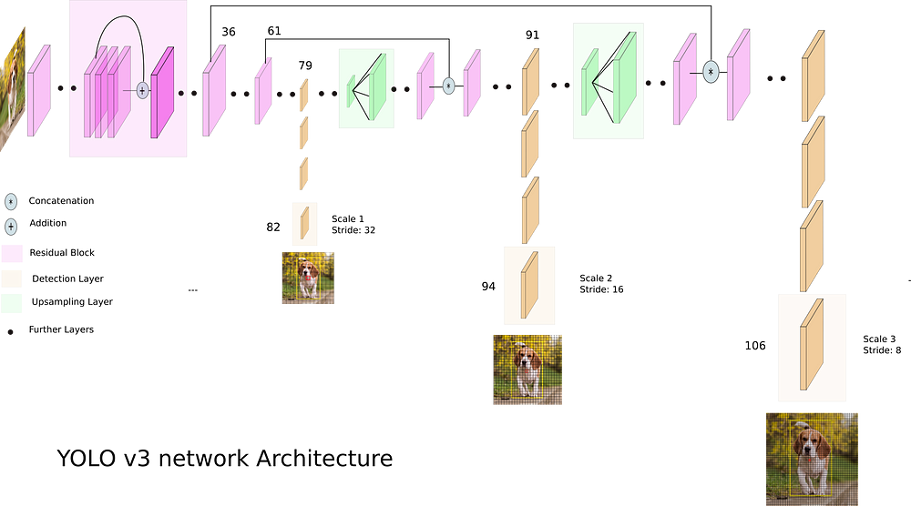
Diagram from What’s new in YOLO v3 by Ayoosh Kathuria

Final word on object detection

• An algorithm like YOLO v3 is somewhat tricky to run
• Preparing the algorithm takes a long time
  • The final output, though, can run on much cheaper hardware
• These algorithms just recently became feasible so their impact has yet to be felt so strongly

Think about how facial recognition showed up everywhere for images over the past few years

Where to get video data

• One extensive source is Youtube-8M
  • 6.1M videos, 3-10 minutes each
  • Each video has >1,000 views
  • 350,000 hours of video
  • 237,000 labeled 5 second segments
  • 1.3B video features that are machine labeled
  • 1.3B audio features that are machine labeled

A word on ethics of object detection

From Redmon and Farhadi (2018) [The YOLO v3 paper]

Combining images and text in 1 model

Large language models + Images

• Multiple impactful models were released since 2021 that merge text and image processing into a single model
  • CLIP: Contrastive Language-Image Pre-training
    • Pairs images with captions
  • Stable Diffusion
    • Image generation from text

These work by embedding images and text into the same embedding space

CLIP

• Code for this is available at: rmc.link/colab_clip

Stable diffusion: Content

• Code to implement as a Telegram bot: rmcrowley2000/StableDiffBot

“A photo of the Singapore skyline including Marina Bay Sands”

“Singapore Management University”

Stable diffusion: Style

“Lithograph of a camel eating a pear”

“A cartoon icon of a dog getting a hair cut.”

Stable diffusion: Problems

“Sustainability data”

“A cavapoo enjoying a nice warm cup of tea”

Stable diffusion: Complexity

“Tiny cute isometric living room in a cutaway box, soft smooth lighting, soft colors, purple and blue color scheme, soft colors, 100mm lens, 3d blender render”

End Matter

Recap

Today, we:

• Learned about using images as data
• Constructed a simple handwriting recognition system
• Learned about more advanced image methods
• Applied CNNs to detect financial information in images on Twitter
• Learned about object detection in videos
• Learned about methods combining images and text

Wrap up

• For next week:
  • Finish the group project!
    1. Kaggle submission closes Monday!
    2. Turn in your code, presentation, and report through eLearn’s dropbox
    3. Prepare a short (~12-15 minute) presentation for class
• Survey on the class session at this QR code:

More fun examples

• Interactive:
  • Performance RNN
  • TensorFlow.js examples
• Others:
  • Google’s deepdream
  • Open NSynth Super

Bonus: Neural networks in interactive media

• Super Mario using MarI/O
• Mario Kart using an RNN for controller prediction
• Open AI’s Five tops Dota 2
  • Trained on 180 years of play
• Google Deepmind’s Alphastar AI on StarCraft II
  • Trained on 200 years of play

Packages used for these slides

• DT
• downlit
• kableExtra
• keras
• knitr
• plotly
• quarto
• revealjs
• tidyverse