ACCT 420: Logistic Regression

Dr. Richard M. Crowley

rcrowley@smu.edu.sg

https://rmc.link/

Front Matter

Learning objectives

Roadmap for the course

Theory:
- Understanding binary problems
Application:
- Detecting shipping delays caused by typhoons
Methodology:
- Logistic regression
- Spatial visualization

Assignment 2

Looking at Singaporean retail firms
- Mostly focused on time and cyclicality
- Some visualization
- A little of what we cover today
Optional (but encouraged):
- You can work in pairs on this assignment
  - If you choose to do this, please only make 1 submission and include both your names on the submission

Binary outcomes

What are binary outcomes?

Thus far we have talked about events with continuous outcomes
- Revenue: Some positive number
- Earnings: Some number
- ROA: Some percentage
Binary outcomes only have two possible outcomes
- Did something happen, yes or no?
- Is a statement true or false?

Accounting examples of binary outcomes

Financial accounting:
- Will the company’s earnings meet analysts’ expectations?
- Will the company have positive earnings?
Managerial accounting:
- Will we have ___ problem with our supply chain?
- Will our customer go bankrupt?
Audit:
- Is the company committing fraud?
Taxation:
- Is the company too aggressive in their tax positions?

We can assign a probability to any of these

Brainstorming…

What types of business problems or outcomes are binary?

Regression approach: Logistic regression

When modeling a binary outcome, we use logistic regression
- A.k.a. logit model
The logit function is \(logit(x) = \text{log}\left(\frac{x}{1-x}\right)\)
- Also called log odds

\[ \text{log}\left(\frac{\text{Prob}(y=1|X)}{1-\text{Prob}(y=1|X)}\right)=\alpha + \beta_1 x_1 + \beta_2 x_2 + \ldots + \varepsilon \]

There are other ways to model this though, such as probit

Implementation: Logistic regression

The logistic model is related to our previous linear models as such:

Both linear and logit models are under the class of General Linear Models (GLMs)

To regress a GLM, we use the glm() command.
- In fact, the lm() command we have been using is actually glm() when you specify the option family=gaussian
To run a logit regression:

mod <- glm(y ~ x1 + x2 + x3 + ..., data=df, family=binomial)

summary(mod)

family=binomial is what sets the model to be a logit

Interpreting logit values

The sign of the coefficients means the same as before
- +: increases the likelihood of \(y\) occurring
- -: decreases the likelihood of \(y\) occurring
The level of a coefficient is different
- The relationship isn’t linear between \(x_i\) and \(y\) now
- Instead, coefficients are in log odds
  - Thus, \(e^{\beta_i}\) gives you the odds, \(o\)
You can interpret the odds for a coefficient
- Increased by \([o-1]\%\)
You need to sum all relevant log odds before converting to a probability!

Odds vs probability

Example logit regression

Do holidays increase the likelihood that a department more than doubles its store’s average weekly sales across departments?

# Create the binary variable from Walmart sales data
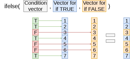
df <- df %>% mutate(double = ifelse(Weekly_Sales > store_avg*2,1,0))
fit <- glm(double ~ IsHoliday, data=df, family=binomial)
tidy(fit)

# A tibble: 2 × 5
  term          estimate std.error statistic  p.value
  <chr>            <dbl>     <dbl>     <dbl>    <dbl>
1 (Intercept)     -3.45    0.00924    -373.  0       
2 IsHolidayTRUE    0.539   0.0278       19.4 1.09e-83

Holidays increase the odds… but by how much?

Logistic regression interpretation

A simple interpretation

The model we just saw the following model:

\[ logodds(Double~sales) = -3.45 + 0.54 IsHoliday \]

There are two ways to interpret this:
1. Coefficient by coefficient
2. In total

Interpretting specific coefficients

\[ logodds(Double~sales) = -3.45 + 0.54 IsHoliday \]

Interpreting specific coefficients is easiest done manually
Odds for the \(IsHoliday\) coefficient are exp(0.54) = 1.72
- This means that having a holiday modifies the baseline (i.e., non-Holiday) odds by 1.72 to 1
  - Where 1 to 1 is considered no change
- Baseline is 0.032 to 1

# Automating the above:
exp(coef(fit))

  (Intercept) IsHolidayTRUE 
   0.03184725    1.71367497

Interpretting in total

It is important to note that log odds are additive
- So, calculate a new log odd by plugging in values for variables and adding it all up
  - Holiday: \(-3.45 + 0.54 * 1 = -2.89\)
  - No holiday: \(-3.45 + 0.54 * 0 = -3.45\)
Then calculate odds and log odds like before
- With holiday: exp(-2.89) = 0.056
- Without holiday: exp(-3.45) = 0.032
- Ratio of holiday to without: 1.72!
  - This is the individual log odds for holiday

We need to specify values to calculate log odds in total

Converting to probabilities

We can calculate a probability at any given point using the log odds

\[ Probability = \frac{odds}{odds + 1} \]

Probability of double sales…
- With a holiday: 0.056 / (0.056 + 1) = 0.052
- Without a holiday: 0.032 / (0.032 + 1) = 0.031

These are easier to interpret, but require specifying values for each model input to calculate

Using `predict()` to simplify it

predict() can calculate log odds and probabilities for us with minimal effort
- Specify type="response" to get probabilities

Outcomes

test_data <- data.frame(IsHoliday = c(F,T))
predict(fit, test_data)  # log odds

        1         2 
-3.446804 -2.908164

# probabilities
predict(fit, test_data, type="response")

         1          2 
0.03086431 0.05175146

Converting from log odds to probabilities

a <- exp(-3.446804)
b <- exp(-2.908164)
c(a/(1+a), b/(1+b))

[1] 0.03086431 0.05175146

Here, we see the baseline probability is 3.1%
The probability of doubling sales on a holiday is higher, at 5.2%

R practice: Logit

A continuation of last week’s practices answering:
- Is Walmart more likely to see a year over year decrease in quarterly revenue during a recession?
Practice using mutate() and glm()
Do exercises 1 and 2 in today’s practice file
- R Practice
- Shortlink: rmc.link/420r4

Logistic regression interpretation redux

What about more complex models?

Continuous inputs in the model
- What values do we pick to determine probabilities?
Multiple inputs?
- We can scale up what we did, but things get messy
  - Mathematically, the inputs get interacted within the inner workings of logit…
    - So the impact of each input depends on the values of the others!

Consider this model

fit2 <- glm(double ~ IsHoliday + Temperature + Fuel_Price, data=df, family=binomial)
summary(fit2)


Call:
glm(formula = double ~ IsHoliday + Temperature + Fuel_Price, 
    family = binomial, data = df)

Coefficients:
                Estimate Std. Error z value Pr(>|z|)    
(Intercept)   -1.7764917  0.0673246  -26.39   <2e-16 ***
IsHolidayTRUE  0.3704298  0.0284395   13.03   <2e-16 ***
Temperature   -0.0108268  0.0004698  -23.04   <2e-16 ***
Fuel_Price    -0.3091950  0.0196234  -15.76   <2e-16 ***
---
Signif. codes:  0 '***' 0.001 '**' 0.01 '*' 0.05 '.' 0.1 ' ' 1

(Dispersion parameter for binomial family taken to be 1)

    Null deviance: 120370  on 421569  degrees of freedom
Residual deviance: 119146  on 421566  degrees of freedom
AIC: 119154

Number of Fisher Scoring iterations: 6

Odds and probabilities

# Odds
exp(coef(fit2))

  (Intercept) IsHolidayTRUE   Temperature    Fuel_Price 
    0.1692308     1.4483570     0.9892316     0.7340376

# Typical September days
hday_sep    <- mean(predict(fit2, filter(df, IsHoliday, month==9), type="response"))
no_hday_sep <-  mean(predict(fit2, filter(df, !IsHoliday, month==9), type="response"))
# Typical December days
hday_dec    <- mean(predict(fit2, filter(df, IsHoliday, month==12), type="response"))
no_hday_dec <-  mean(predict(fit2, filter(df, !IsHoliday, month==12), type="response"))

html_df(data.frame(Month=c(9,9,12,12), IsHoliday=c(FALSE,TRUE,FALSE,TRUE),
                   Probability=c(no_hday_sep, hday_sep, no_hday_dec, hday_dec)))

Month	IsHoliday	Probability
9	FALSE	0.0266789
9	TRUE	0.0374761
12	FALSE	0.0398377
12	TRUE	0.0586483

A bit easier: Marginal effects

Marginal effects tell us the average change in our output for a change of 1 to an input

The above definition is very similar to how we interpret linear regression coefficients
- The only difference is the word average – the effect changes a bit depending on the input data
Using margins, we can calculate marginal effects
There are a few types that we could calculate:
- An Average Marginal Effect tells us what the average effect of an input is across all values in our data
  - This is the default method in the package
- We can also specify a specific value to calculate marginal effects at (like with our probabilities last slides)

Marginal effects in action

# Calculate AME marginal effects
library(margins)
m <- margins(fit2)
m

 Temperature Fuel_Price IsHoliday
  -0.0003377  -0.009644   0.01334

A holiday increase the probability of doubling by a flat 1.33%
- Not too bad when you consider that the probability of doubling is 3.23%
If the temperature goes up by 1°F (0.55°C), the probability of doubling changes by -0.03%
If the fuel price increases by 1 USD for 1 gallon of gas, the probability of doubling changes by -0.96%

`margins` niceties

We can get some extra information about our marginal effects through summary():

summary(m) %>%
  html_df()

factor	AME	SE	z	lower	upper
Fuel_Price	-0.0096438	0.0006163	-15.64800	-0.0108517	-0.0084359
IsHoliday	0.0133450	0.0011754	11.35372	0.0110413	0.0156487
Temperature	-0.0003377	0.0000149	-22.71256	-0.0003668	-0.0003085

Those p-values work just like with our linear models
We also get a confidence interval
- Which we can plot!

Plotting marginal effects

plot(m, which=summary(m)$factor)

Note: The which... part is absolutely necessary at the moment due to a bug in the package

Marginal effects at a specified value

margins(fit2, at = list(IsHoliday = c(TRUE, FALSE)),
        variables = c("Temperature", "Fuel_Price")) %>%
  summary() %>%
  html_df()

factor	IsHoliday	AME	SE	z	lower	upper
Fuel_Price	FALSE	-0.0093401	0.0005989	-15.59617	-0.0105139	-0.0081664
Fuel_Price	TRUE	-0.0131335	0.0008717	-15.06650	-0.0148420	-0.0114250
Temperature	FALSE	-0.0003271	0.0000146	-22.46024	-0.0003556	-0.0002985
Temperature	TRUE	-0.0004599	0.0000210	-21.92927	-0.0005010	-0.0004188

margins(fit2, at = list(Temperature = c(0, 25, 50, 75, 100)),
        variables = c("IsHoliday")) %>%
  summary() %>%
  html_df()

factor	Temperature	AME	SE	z	lower	upper
IsHoliday	0	0.0234484	0.0020168	11.62643	0.0194955	0.0274012
IsHoliday	25	0.0184956	0.0015949	11.59704	0.0153697	0.0216214
IsHoliday	50	0.0144798	0.0012679	11.42060	0.0119948	0.0169648
IsHoliday	75	0.0112693	0.0010161	11.09035	0.0092777	0.0132609
IsHoliday	100	0.0087305	0.0008213	10.62977	0.0071207	0.0103402

Today’s Application: Shipping delays

The question

Can we leverage global weather data to predict shipping delays?

Formalization

Question
- How can predict naval shipping delays?
Hypothesis (just the alternative ones)
1. Global weather data helps to predict shipping delays
Prediction
- Use Logistic regression and \(z\)-tests for coefficients
- No hold out sample this week – too little data

A bit about shipping data

WRDS doesn’t have shipping data
There are, however, vendors for shipping data, such as:

They pretty much have any data you could need:
- Over 650,000 ships tracked using ground and satellite based AIS
  - AIS: Automatic Identification System
- Live mapping
- Weather data
- Fleet tracking
- Port congestion
- Inmarsat support for ship operators

What can we see from naval data?

Yachts in the Mediterranean

Oil tankers in the Persian gulf

What can we see from naval data?

Shipping route via the Panama canal

River shipping on the Mississippi river, USA

What can we see from naval data?

Busiest ports by containers and tons (Shanghai & Ningbo-Zhoushan, China)

Busiest port for transshipment (Singapore)

Examining Singaporean owned ships

Code for last slide’s map

library(plotly)  # for plotting
library(RColorBrewer)  # for colors
# plot with boats, ports, and typhoons
# Note: geo is defined in the appendix -- it controls layout
palette = brewer.pal(8, "Dark2")[c(1,8,3,2)]
p <- plot_geo(colors=palette) %>%
  add_markers(data=df_ports, x = ~port_lon, y = ~port_lat, color = "Port") %>%
  add_markers(data=df_Aug31, x = ~lon, y = ~lat, color = ~ship_type,
              text=~paste('Ship name',shipname)) %>%
  add_markers(data=typhoon_Aug31, x = ~lon, y = ~lat, color="TYPHOON",
              text=~paste("Name", typhoon_name)) %>%
   layout(showlegend = TRUE, geo = geo,
    title = 'Singaporean owned container and tanker ships, August 31, 2018')
p

plot_geo() is from plotly
add_markers() adds points to the map
layout() adjusts the layout
Within geo, a list, the following makes the map a globe
- projection=list(type="orthographic")

Singaporean ship movement

Link to ship movement animation

Code for last slide’s map

library(sf)  # Note: very difficult to install except on Windows
library(maps)
# Requires separately installing "maptools" and "rgeos" as well
# This graph requires ~7GB of RAM to render
world1 <- sf::st_as_sf(map('world', plot = FALSE, fill = TRUE))

df_all <- df_all %>% arrange(run, imo)

p <- ggplot(data = world1) + 
  geom_sf() + 
  geom_point(data = df_all, aes(x = lon, y = lat, frame=frame,
                                text=paste("name:",shipname)))
ggplotly(p) %>%
   animation_opts(
    1000, easing = "linear", redraw = FALSE)

world1 contains the map data
geom_sf() plots map data passed to ggplot()
geom_point() plots ship locations as longitude and latitude
ggplotly() converts the graph to html and animates it
- Animation follows the frame aesthetic

Typhoon Jebi

Typhoons in the data

Code for last slide’s map

# plot with boats and typhoons
palette = brewer.pal(8, "Dark2")[c(1,3,2)]
p <- plot_geo(colors=palette) %>%
  add_markers(data=df_all[df_all$frame == 14,], x = ~lon, y = ~lat,
              color = ~ship_type, text=~paste('Ship name',shipname)) %>%
  add_markers(data=typhoon_Jebi, x = ~lon,
              y = ~lat, color="Typhoon Jebi",
              text=~paste("Name", typhoon_name, "</br>Time: ", date)) %>%
   layout(showlegend = TRUE, geo = geo,
    title = 'Singaporean container/tanker ships, September 4, 2018, evening')
p

This map is made the same way as the first map

Typhoons in the data using leaflet

Code for last slide’s map

library(leaflet)
library(leaflet.extras)

# typhoon icons
ty_icons <- pulseIcons(color='red',  #  supports hex colors like "#C0C0C0"
  heartbeat = 1.2,  #heartbeat is frequency of pulsing
  iconSize=3)

# ship icons
shipicons <- iconList(
  ship = makeIcon("../Figures/ship.png", NULL, 18, 18)
)

leaflet() %>%
  addTiles() %>% 
  setView(lng = 136, lat = 20, zoom=3) %>%
  addCircleMarkers(data=typhoon_Jebi[typhoon_Jebi$intensity_vmax <= 150/1.852,], lng=~lon, lat=~lat,  # Not super typhoon
                   stroke = TRUE, radius=2, color="orange", label=~date) %>%
  addPulseMarkers(data=typhoon_Jebi[typhoon_Jebi$intensity_vmax > 150/1.852,], lng=~lon, lat=~lat,  # Super typhoon
                   icon=ty_icons, label=~date) %>%
  addMarkers(data=df_all[df_all$frame == 14,], lng=~lon, lat=~lat,
             label=~shipname, icon=shipicons)

pulseIcons(): pulsing icons from leaflet.extras
iconList(): pulls icons stored on your computer
leaflet(): start the map; addTiles() pulls from OpenStreetMap
setView(): sets the frame for the map
addPulseMarkers(): adds pulsing markers
addCircleMarkers(): adds circular markers

R Practice on mapping

Practice mapping typhoon data
- 1 map using plotly
- 1 map using leaflet
Practice using plotly and leaflet
No practice using ggplot2 with sf
- The technical difficulties involved in setting up sf, along with the computational intensity, make it a bit tricky
Do exercises 3 and 4 in today’s practice file
- R Practice
- Shortlink: rmc.link/420r4

Predicting delays due to typhoons

Data

If the ship will report a delay of at least 3 hours some time in the next 12-24 hours
What we have:
- Ship location
- Typhoon location
- Typhoon wind speed

We need to calculate distance between ships and typhoons

Distance for geo

Use st_distance() from sf to get a quick and reasonably accurate calculation
- Uses great-circle distance

library(sf)

# sf can't handle NA values, so we need to filter them out
df3 <- df3 %>% mutate(n = row_number())
df_ty <- df3 %>% filter(!is.na(ty_lat), !is.na(ty_lon))

# Create lists of points on Earth
x <- st_as_sf(df_ty %>% select("lon", "lat"), coords = c("lon", "lat"), 
                 crs = 4326, agr = "constant")
y <- st_as_sf(df_ty %>% select("ty_lon", "ty_lat"), coords = c("ty_lon", "ty_lat"), 
                 crs = 4326, agr = "constant")

# Find the distance between the points
df_ty$dist_typhoon <- st_distance(x, y, by_element=T) / 1000  # distance in km

# Add the distance back to our main data
# Replaced NAs with a placeholder longer than any possible distance
df3 <- df3 %>%
  left_join(df_ty %>% select(n, dist_typhoon)) %>%
  mutate(dist_typhoon = ifelse(is.na(dist_typhoon), 20036, dist_typhoon)) %>%
  select(-n)

The st_distance() function is not 100% accurate

The great-circle distance function assumes the Earth is a sphere. As such, for some distances it is off by ~0.5%. A better approach is Vincenty’s Formula, but the R package for calculating this is deprecated as of October 2023.

Clean up

Some indicators to cleanly capture how far away the typhoon is

df3$typhoon_500 = ifelse(df3$dist_typhoon < 500 & 
                         df3$dist_typhoon >= 0, 1, 0)
df3$typhoon_1000 = ifelse(df3$dist_typhoon < 1000 &
                          df3$dist_typhoon >= 500, 1, 0)
df3$typhoon_2000 = ifelse(df3$dist_typhoon < 2000 &
                          df3$dist_typhoon >= 1000, 1, 0)

Do typhoons delay shipments?

fit1 <- glm(delayed ~ typhoon_500 + typhoon_1000 + typhoon_2000, data=df3,
            family=binomial)
summary(fit1)


Call:
glm(formula = delayed ~ typhoon_500 + typhoon_1000 + typhoon_2000, 
    family = binomial, data = df3)

Coefficients:
             Estimate Std. Error  z value Pr(>|z|)    
(Intercept)  -3.65381    0.02931 -124.653   <2e-16 ***
typhoon_500   0.14376    0.16311    0.881   0.3781    
typhoon_1000  0.20682    0.12575    1.645   0.1000    
typhoon_2000  0.15681    0.07116    2.203   0.0276 *  
---
Signif. codes:  0 '***' 0.001 '**' 0.01 '*' 0.05 '.' 0.1 ' ' 1

(Dispersion parameter for binomial family taken to be 1)

    Null deviance: 14340  on 59255  degrees of freedom
Residual deviance: 14333  on 59252  degrees of freedom
  (3795 observations deleted due to missingness)
AIC: 14341

Number of Fisher Scoring iterations: 6

It appears so!

Interpretation of coefficients

odds1 <- exp(coef(fit1))
odds1

 (Intercept)  typhoon_500 typhoon_1000 typhoon_2000 
  0.02589235   1.15460211   1.22975514   1.16976795

Ships 1,000 to 2,000 km from a typhoon have a 17% increased odds of having a delay

m1 <- margins(fit1)
summary(m1)

       factor    AME     SE      z      p   lower  upper
 typhoon_1000 0.0053 0.0032 1.6435 0.1003 -0.0010 0.0115
 typhoon_2000 0.0040 0.0018 2.2006 0.0278  0.0004 0.0075
  typhoon_500 0.0037 0.0042 0.8811 0.3782 -0.0045 0.0118

Ships 1,000 to 2,000 km from a typhoon have an extra 0.4% chance of having a delay (baseline of 2.61%)

What about typhoon intensity?

Hong Kong’s typhoon classification: Official source
1. 41-62 km/h: Tropical depression
2. 63-87 km/h: Tropical storm
3. 88-117 km/h: Severe tropical storm
4. 118-149 km/h: Typhoon
5. 150-184 km/h: Severe typhoon
6. 185+km/h: Super typhoon

# Cut makes a categorical variable out of a numerical variable using specified bins
df3$Super <- ifelse(df3$intensity_vmax * 1.852 > 185, 1, 0)
df3$Moderate <- ifelse(df3$intensity_vmax * 1.852 >= 88 &
                         df3$intensity_vmax * 1.852 < 185, 1, 0)
df3$Weak <- ifelse(df3$intensity_vmax * 1.852 >= 41 & 
                   df3$intensity_vmax * 1.852 < 88, 1, 0)
df3$HK_intensity <- cut(df3$intensity_vmax * 1.852 ,c(-1,41, 62, 87, 117, 149, 999))
table(df3$HK_intensity)


  (-1,41]   (41,62]   (62,87]  (87,117] (117,149] (149,999] 
     3398     12039     12615     11527      2255     21141

Typhoon intensity and delays

fit2 <- glm(delayed ~ (typhoon_500 + typhoon_1000 + typhoon_2000) : 
              (Weak + Moderate + Super), data=df3,
            family=binomial)
tidy(fit2)

# A tibble: 10 × 5
   term                  estimate std.error statistic p.value
   <chr>                    <dbl>     <dbl>     <dbl>   <dbl>
 1 (Intercept)           -3.65       0.0290 -126.     0      
 2 typhoon_500:Weak      -0.00723    0.213    -0.0339 0.973  
 3 typhoon_500:Moderate   0.718      0.251     2.86   0.00417
 4 typhoon_500:Super     -8.91     123.       -0.0726 0.942  
 5 typhoon_1000:Weak      0.251      0.161     1.56   0.120  
 6 typhoon_1000:Moderate  0.120      0.273     0.441  0.659  
 7 typhoon_1000:Super    -0.0191     0.414    -0.0461 0.963  
 8 typhoon_2000:Weak      0.169      0.101     1.66   0.0963 
 9 typhoon_2000:Moderate  0.0260     0.134     0.194  0.846  
10 typhoon_2000:Super     0.316      0.136     2.33   0.0198

Moderate storms predict delays when within 500km

Super typhoons predict delays when 1,000 to 2,000km away

Interpretation of coefficients

m2 <- margins(fit2)
summary(m2) %>%
  html_df()

factor	AME	SE	z	p	lower	upper
Moderate	0.0007384	0.0006695	1.1028719	0.2700828	-0.0005738	0.0020505
Super	-0.0049982	0.0859612	-0.0581445	0.9536336	-0.1734789	0.1634826
typhoon_1000	0.0035770	0.0036204	0.9880155	0.3231451	-0.0035188	0.0106727
typhoon_2000	0.0038115	0.0017865	2.1334568	0.0328873	0.0003100	0.0073130
typhoon_500	-0.0440770	0.6812520	-0.0647000	0.9484129	-1.3793065	1.2911525
Weak	0.0009451	0.0005135	1.8404065	0.0657086	-0.0000614	0.0019515

Delays appear to be driven mostly by 2 factors:
1. A typhoon 1,000 to 2,000 km away from the ship
2. Weak typhoons

Interpretating interactions

factor	Weak	AME	SE	z	p	lower	upper
typhoon_1000	1	0.0073448	0.0053623	1.3697146	0.1707760	-0.0031651	0.0178547
typhoon_2000	1	0.0063950	0.0031242	2.0469359	0.0406644	0.0002717	0.0125182
typhoon_500	1	-0.0457062	0.7044878	-0.0648786	0.9482707	-1.4264768	1.3350645

factor	Moderate	AME	SE	z	p	lower	upper
typhoon_1000	1	0.0059123	0.0078242	0.7556384	0.4498660	-0.0094229	0.0212474
typhoon_2000	1	0.0043822	0.0039442	1.1110625	0.2665414	-0.0033482	0.0121126
typhoon_500	1	-0.0311833	0.6856382	-0.0454807	0.9637241	-1.3750095	1.3126429

factor	Super	AME	SE	z	p	lower	upper
typhoon_1000	1	0.0032538	0.0111428	0.2920086	0.7702801	-0.0185858	0.0250934
typhoon_2000	1	0.0102396	0.0041602	2.4613510	0.0138415	0.0020858	0.0183934
typhoon_500	1	-0.2242811	3.1633421	-0.0709000	0.9434773	-6.4243176	5.9757554

What might matter for shipping?

What other observable events or data might provide insight as to whether a naval shipment will be delayed or not?

What is the reason that this event or data would be useful in predicting delays?
- I.e., how does it fit into your mental model?

End Matter

Wrap up

For next week:
- Finish the first individual assignment
- Second individual assignment
  - Finish by 2 classes from now
  - Submit on eLearn
- Think about who you want to work with for the project
Survey on the class session at this QR code:

Packages used for these slides

Custom code

# styling for plotly maps
geo <- list(
  showland = TRUE,
  showlakes = TRUE,
  showcountries = TRUE,
  showocean = TRUE,
  countrywidth = 0.5,
  landcolor = toRGB("grey90"),
  lakecolor = toRGB("aliceblue"),
  oceancolor = toRGB("aliceblue"),
  projection = list(
    type = 'orthographic',  # detailed at https://plot.ly/r/reference/#layout-geo-projection
    rotation = list(
      lon = 100,
      lat = 1,
      roll = 0
    )
  ),
  lonaxis = list(
    showgrid = TRUE,
    gridcolor = toRGB("gray40"),
    gridwidth = 0.5
  ),
  lataxis = list(
    showgrid = TRUE,
    gridcolor = toRGB("gray40"),
    gridwidth = 0.5
  )
)

ACCT 420: Logistic Regression

Front Matter

Learning objectives

Assignment 2

Binary outcomes

What are binary outcomes?

Accounting examples of binary outcomes

Brainstorming…

Regression approach: Logistic regression

Implementation: Logistic regression

Interpreting logit values

Odds vs probability

Example logit regression

Logistic regression interpretation

A simple interpretation

Interpretting specific coefficients

Interpretting in total

Converting to probabilities

Using predict() to simplify it

R practice: Logit

Logistic regression interpretation redux

What about more complex models?

Consider this model

Odds and probabilities

A bit easier: Marginal effects

Marginal effects in action

margins niceties

Plotting marginal effects

Marginal effects at a specified value

Today’s Application: Shipping delays

The question

Formalization

A bit about shipping data

What can we see from naval data?

What can we see from naval data?

What can we see from naval data?

Examining Singaporean owned ships

Code for last slide’s map

Singaporean ship movement

Code for last slide’s map

Typhoon Jebi

Typhoons in the data

Code for last slide’s map

Typhoons in the data using leaflet

Code for last slide’s map

R Practice on mapping

Predicting delays due to typhoons

Data

Distance for geo

Clean up

Do typhoons delay shipments?

Interpretation of coefficients

What about typhoon intensity?

Typhoon intensity and delays

Interpretation of coefficients

Interpretating interactions

What might matter for shipping?

End Matter

Wrap up

Packages used for these slides

Custom code

Using `predict()` to simplify it

`margins` niceties