ACCT 420: Logistic Regression
Session 5
Dr. Richard M. Crowley
Front matter
Learning objectives

- Theory:
- Further understand:
- Binary problems
- Further understand:
- Application:
- Detecting shipping delays caused by typhoons
- Methodology:
- Logistic regression
Datacamp
- Explore on your own
- No specific required class this week
Assignment 2
- Looking at Singaporean retail firms
- Mostly focused on time and cyclicality
- Some visualization
- A little of what we cover today
- Optional:
- You can work in pairs on the homework.
- If you choose to do this, please only make 1 submission and include both your names on the submission
- You can work in pairs on the homework.
Weekly revenue prediction
Shifted from week 4
The question
How can we weekly departmental revenue for Walmart, leveraging our knowledge of Walmart, its business, and some limited historical information
- Predict weekly for 115,064 (Store, Department, Week) tuples
- From 2012-11-02 to 2013-07-26
- Using [incomplete] weekly revenue data from 2010-02-015 to 2012-10-26
- By department (some weeks missing for some departments)
More specifically…
- Consider time dimensions
- What matters:
- Time of the year?
- Holidays?
- Do different stores or departments behave differently?
- What matters:
- Wrinkles:
- Walmart won’t give us testing data
- But they’ll tell us how well the algorithm performs
- We can’t use past week sales for prediction because we won’t have it for most of the prediction…
- Walmart won’t give us testing data
The data
- Revenue by week for each department of each of 45 stores
- Department is just a number between 1 and 99
- Date of that week
- If the week is considered a holiday for sales purposes
- Super Bowl, Labor Day, Black Friday, Christmas
- Store data:
- Which store the data is for, 1 to 45
- Store type (A, B, or C)
- Store size
- Other data, by week and location:
- Temperature, gas price, sales (by department), CPI, Unemployment, Holidays
Walmart’s evaluation metric
- Walmart uses MAE (mean absolute error), but with a twist:
- They care more about holidays, so any error on holidays has 5 times the penalty
- They call this WMAE, for weighted mean absolute error
WMAE = \frac{1}{\sum w_i} \sum_{i=1}^{n} w_i \left|y_i-\hat{y}_i\right|
- n is the number of test data points
- \hat{y}_i is your prediction
- y_i is the actual sales
- w_i is 5 on holidays and 1 otherwise
wmae <- function(actual, predicted, holidays) {
  sum(abs(actual-predicted)*(holidays*4+1)) / (length(actual) + 4*sum(holidays))
}
Before we get started…
- The data isn’t very clean:
- Markdowns are given by 5 separate variables instead of 1
- Date is text format instead of a date
- CPI and unemployment data are missing in around a third of the testing data
- There are some (week, store, department) groups missing from our training data!
We’ll have to fix these
Also…
- Some features to add:
- Year
- Week
- A unique ID for tracking (week, firm, department) tuples
- The ID Walmart requests we use for submissions
- Average sales by (store, department)
- Average sales by (week, store, department)
Load data and packages
library(tidyverse)  # we'll extensively use dplyr here
library(lubridate)  # Great for simple date functions
library(broom)
weekly <- read.csv("../../Data/WMT_train.csv", stringsAsFactors=FALSE)
weekly.test <- read.csv("../../Data/WMT_test.csv", stringsAsFactors=FALSE)
weekly.features <- read.csv("../../Data/WMT_features.csv", stringsAsFactors=FALSE)
weekly.stores <- read.csv("../../Data/WMT_stores.csv", stringsAsFactors=FALSE)weeklyis our training dataweekly.testis our testing data – noWeekly_Salescolumnweekly.featuresis general information about (week, store) pairs- Temperature, pricing, etc.
weekly.storesis general information about each store
Cleaning
preprocess_data <- function(df) {
  # Merge the data together (Pulled from outside of function -- "scoping")
  df <- inner_join(df, weekly.stores)
  df <- inner_join(df, weekly.features[,1:11])

  # Compress the weird markdown information to 1 variable
  df$markdown <- 0
  df[!is.na(df$MarkDown1),]$markdown <- df[!is.na(df$MarkDown1),]$MarkDown1
  df[!is.na(df$MarkDown2),]$markdown <- df[!is.na(df$MarkDown2),]$MarkDown2
  df[!is.na(df$MarkDown3),]$markdown <- df[!is.na(df$MarkDown3),]$MarkDown3
  df[!is.na(df$MarkDown4),]$markdown <- df[!is.na(df$MarkDown4),]$MarkDown4
  df[!is.na(df$MarkDown5),]$markdown <- df[!is.na(df$MarkDown5),]$MarkDown5

  # Fix dates and add useful time variables
  df$date <- as.Date(df$Date)
  df$week <- week(df$date)
  df$year <- year(df$date)

  df
}
df <- preprocess_data(weekly)
df_test <- preprocess_data(weekly.test)Merge data, fix
markdown, build time data
What this looks like
df[91:94,] %>%
  select(Store, date, markdown, MarkDown3, MarkDown4, MarkDown5) %>%
html_df()| Store | date | markdown | MarkDown3 | MarkDown4 | MarkDown5 | |
|---|---|---|---|---|---|---|
| 91 | 1 | 2011-10-28 | 0.00 | NA | NA | NA |
| 92 | 1 | 2011-11-04 | 0.00 | NA | NA | NA |
| 93 | 1 | 2011-11-11 | 6551.42 | 215.07 | 2406.62 | 6551.42 |
| 94 | 1 | 2011-11-18 | 5988.57 | 51.98 | 427.39 | 5988.57 |
df[1:2,] %>% select(date, week, year) %>% html_df()| date | week | year |
|---|---|---|
| 2010-02-05 | 6 | 2010 |
| 2010-02-12 | 7 | 2010 |
Cleaning: Missing CPI and Unemployment
# Fill in missing CPI and Unemployment data
df_test <- df_test %>%
  group_by(Store, year) %>%
  mutate(CPI=ifelse(is.na(CPI), mean(CPI,na.rm=T), CPI),
         Unemployment=ifelse(is.na(Unemployment),
                             mean(Unemployment,na.rm=T),
                             Unemployment)) %>%
  ungroup()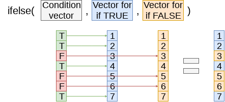
Apply the (year, Store)’s CPI and Unemployment to missing data
Cleaning: Adding IDs
- Build a unique ID
- Since Store, week, and department are all 2 digits, make a 6 digit number with 2 digits for each
sswwdd
- Since Store, week, and department are all 2 digits, make a 6 digit number with 2 digits for each
- Build Walmart’s requested ID for submissions
ss_dd_YYYY-MM-DD
# Unique IDs in the data
df$id <- df$Store *10000 + df$week * 100 + df$Dept
df_test$id <- df_test$Store *10000 + df_test$week * 100 + df_test$Dept

# Unique ID and factor building
swd <- c(df$id, df_test$id)  # Pool all IDs
swd <- unique(swd)  # Only keep unique elements
swd <- data.frame(id=swd)  # Make a data frame
swd$swd <- factor(swd$id)  # Extract factors for using later

# Add unique factors to data -- ensures same factors for both data sets
df <- left_join(df,swd)
df_test <- left_join(df_test,swd)df_test$Id <- paste0(df_test$Store,'_',df_test$Dept,"_",df_test$date)What the IDs look like
html_df(df_test[c(20000,40000,60000),c("Store","week","Dept","id","swd","Id")])| Store | week | Dept | id | swd | Id |
|---|---|---|---|---|---|
| 8 | 27 | 33 | 82733 | 82733 | 8_33_2013-07-05 |
| 15 | 46 | 91 | 154691 | 154691 | 15_91_2012-11-16 |
| 23 | 52 | 25 | 235225 | 235225 | 23_25_2012-12-28 |
Add in (store, department) average sales
# Calculate average by store-dept and distribute to df_test
df <- df %>%
  group_by(Store, Dept) %>%
  mutate(store_avg=mean(Weekly_Sales, rm.na=T)) %>%
  ungroup()
df_sa <- df %>%
  group_by(Store, Dept) %>%
  slice(1) %>%
  select(Store, Dept, store_avg) %>%
  ungroup()
df_test <- left_join(df_test, df_sa)
## Joining, by = c("Store", "Dept")# 36 observations have messed up department codes -- ignore (set to 0)
df_test[is.na(df_test$store_avg),]$store_avg <- 0
# Calculate multipliers based on store_avg (and removing NaN and Inf)
df$Weekly_mult <- df$Weekly_Sales / df$store_avg
df[!is.finite(df$Weekly_mult),]$Weekly_mult <- NAAdd in (week, store, dept) average sales
# Calculate mean by week-store-dept and distribute to df_test
df <- df %>%
  group_by(Store, Dept, week) %>%
  mutate(naive_mean=mean(Weekly_Sales, rm.na=T)) %>%
  ungroup()
df_wm <- df %>%
  group_by(Store, Dept, week) %>%
  slice(1) %>%
  ungroup() %>%
  select(Store, Dept, week, naive_mean)
df_test <- df_test %>% arrange(Store, Dept, week)
df_test <- left_join(df_test, df_wm)
## Joining, by = c("Store", "Dept", "week")ISSUE: New (week, store, dept) groups
- This is in our testing data!
- So we’ll need to predict out groups we haven’t observed at all
table(is.na(df_test$naive_mean))##
## FALSE TRUE
## 113827 1237- Fix: Fill with 1 or 2 lags where possible using ifelse() and lag()
- Fix: Fill with 1 or 2 leads where possible using ifelse() and lag()
- Fill with
store_avgwhen the above fail - Code is available in the code file – a bunch of code like:
df_test <- df_test %>%
  arrange(Store, Dept, date) %>%
  group_by(Store, Dept) %>%
  mutate(naive_mean=ifelse(is.na(naive_mean), lag(naive_mean),naive_mean)) %>%
  ungroup()
Cleaning is done
- Data is in order
- No missing values where data is needed
- Needed values created
df %>%
  group_by(week, Store) %>%
  mutate(sales=mean(Weekly_Sales)) %>%
  slice(1) %>%
  ungroup() %>%
  ggplot(aes(y=sales, x=week, color=factor(Store))) +
  geom_line() + xlab("Week") + ylab("Sales for Store (dept average)") +
  theme(legend.position="none")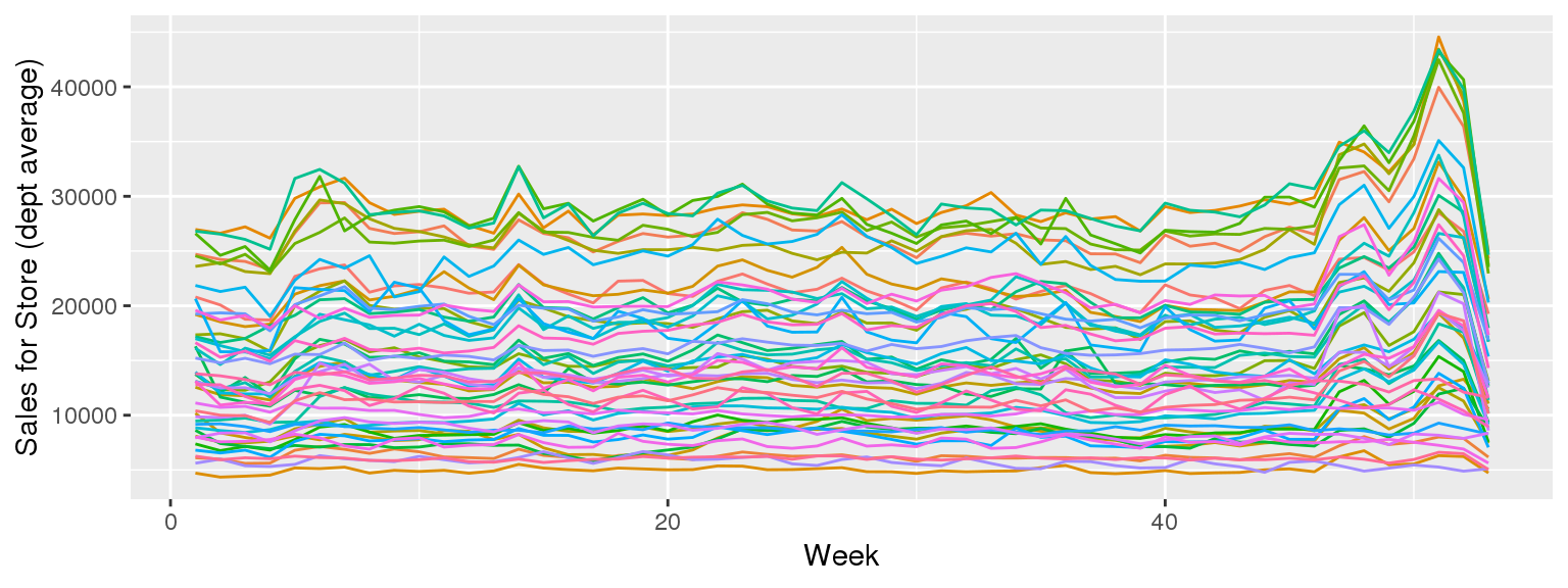
Tackling the problem
First try
- Ideal: Use last week top predict next week!
- Like week 3

No data for testing…
- First instinct: try to use a linear regression to solve this
- Like from week 3

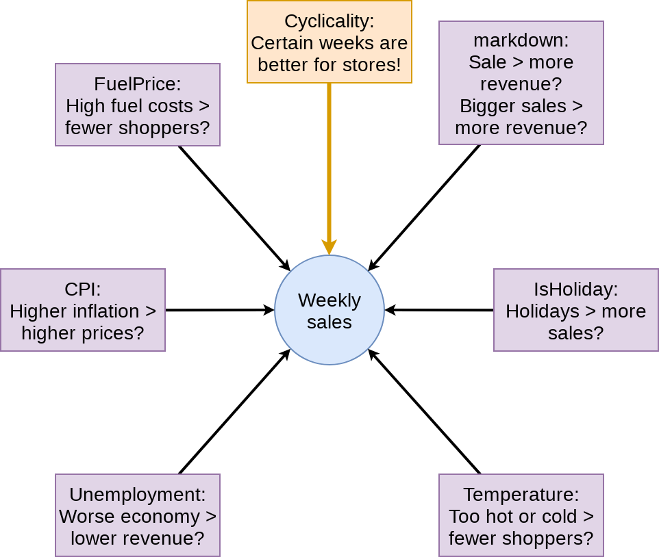
We have this
What to put in the model?
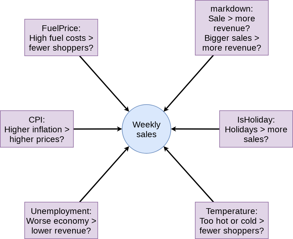
First model
mod1 <- lm(Weekly_mult ~ factor(IsHoliday) + factor(markdown>0) +
                         markdown + Temperature +
                         Fuel_Price + CPI + Unemployment,
           data=df)
tidy(mod1)
## # A tibble: 8 x 5
## term estimate std.error statistic p.value
## <chr> <dbl> <dbl> <dbl> <dbl>
## 1 (Intercept) 1.24 0.0370 33.5 4.10e-245
## 2 factor(IsHoliday)TRUE 0.0868 0.0124 6.99 2.67e- 12
## 3 factor(markdown > 0)TRUE 0.0531 0.00885 6.00 2.00e- 9
## 4 markdown 0.000000741 0.000000875 0.847 3.97e- 1
## 5 Temperature -0.000763 0.000181 -4.23 2.38e- 5
## 6 Fuel_Price -0.0706 0.00823 -8.58 9.90e- 18
## 7 CPI -0.0000837 0.0000887 -0.944 3.45e- 1
## 8 Unemployment 0.00410 0.00182 2.25 2.45e- 2glance(mod1)## # A tibble: 1 x 11
## r.squared adj.r.squared sigma statistic p.value df logLik AIC
## * <dbl> <dbl> <dbl> <dbl> <dbl> <int> <dbl> <dbl>
## 1 0.000481 0.000464 2.03 29.0 2.96e-40 8 -8.96e5 1.79e6
## # ... with 3 more variables: BIC <dbl>, deviance <dbl>, df.residual <int>Prep submission and check in sample WMAE
# Out of sample result
df_test$Weekly_mult <- predict(mod1, df_test)
df_test$Weekly_Sales <- df_test$Weekly_mult * df_test$store_avg

# Required to submit a csv of Id and Weekly_Sales
write.csv(df_test[,c("Id","Weekly_Sales")],
          "WMT_linear.csv",
          row.names=FALSE)

# track
df_test$WS_linear <- df_test$Weekly_Sales

# Check in sample WMAE
df$WS_linear <- predict(mod1, df) * df$store_avg
w <- wmae(actual=df$Weekly_Sales, predicted=df$WS_linear, holidays=df$IsHoliday)
names(w) <- "Linear"
wmaes <- c(w)
wmaes
## Linear
## 3073.57Visualizing in sample WMAE
wmae_obs <- function(actual, predicted, holidays) {
  abs(actual-predicted)*(holidays*5+1) / (length(actual) + 4*sum(holidays))
}
df$wmaes  <- wmae_obs(actual=df$Weekly_Sales, predicted=df$WS_linear,
                      holidays=df$IsHoliday)
ggplot(data=df, aes(y=wmaes, x=week, color=factor(IsHoliday))) +
  geom_jitter(width=0.25) + xlab("Week") + ylab("WMAE")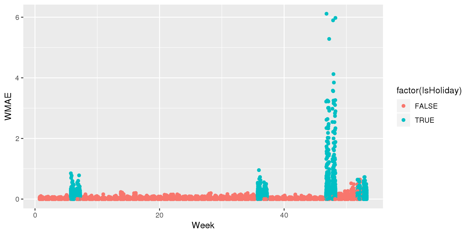
Back to the drawing board…
Second model: Including week
mod2 <- lm(Weekly_mult ~ factor(week) + factor(IsHoliday) + factor(markdown>0) +
                         markdown + Temperature +
                         Fuel_Price + CPI + Unemployment,
           data=df)
tidy(mod2)
## # A tibble: 60 x 5
## term estimate std.error statistic p.value
## <chr> <dbl> <dbl> <dbl> <dbl>
## 1 (Intercept) 1.000 0.0452 22.1 3.11e-108
## 2 factor(week)2 -0.0648 0.0372 -1.74 8.19e- 2
## 3 factor(week)3 -0.169 0.0373 -4.54 5.75e- 6
## 4 factor(week)4 -0.0716 0.0373 -1.92 5.47e- 2
## 5 factor(week)5 0.0544 0.0372 1.46 1.44e- 1
## 6 factor(week)6 0.161 0.0361 4.45 8.79e- 6
## 7 factor(week)7 0.265 0.0345 7.67 1.72e- 14
## 8 factor(week)8 0.109 0.0340 3.21 1.32e- 3
## 9 factor(week)9 0.0823 0.0340 2.42 1.55e- 2
## 10 factor(week)10 0.101 0.0341 2.96 3.04e- 3
## # ... with 50 more rowsglance(mod2)## # A tibble: 1 x 11
## r.squared adj.r.squared sigma statistic p.value df logLik AIC
## * <dbl> <dbl> <dbl> <dbl> <dbl> <int> <dbl> <dbl>
## 1 0.00501 0.00487 2.02 35.9 0 60 -8.95e5 1.79e6
## # ... with 3 more variables: BIC <dbl>, deviance <dbl>, df.residual <int>Prep submission and check in sample WMAE
# Out of sample result
df_test$Weekly_mult <- predict(mod2, df_test)
df_test$Weekly_Sales <- df_test$Weekly_mult * df_test$store_avg

# Required to submit a csv of Id and Weekly_Sales
write.csv(df_test[,c("Id","Weekly_Sales")],
          "WMT_linear2.csv",
          row.names=FALSE)

# track
df_test$WS_linear2 <- df_test$Weekly_Sales

# Check in sample WMAE
df$WS_linear2 <- predict(mod2, df) * df$store_avg
w <- wmae(actual=df$Weekly_Sales, predicted=df$WS_linear2, holidays=df$IsHoliday)
names(w) <- "Linear 2"
wmaes <- c(wmaes, w)
wmaes
## Linear Linear 2
## 3073.570 3230.643Visualizing in sample WMAE
df$wmaes  <- wmae_obs(actual=df$Weekly_Sales, predicted=df$WS_linear2,
                      holidays=df$IsHoliday)
ggplot(data=df, aes(y=wmaes,
                    x=week,
                    color=factor(IsHoliday))) +
  geom_jitter(width=0.25) + xlab("Week") + ylab("WMAE")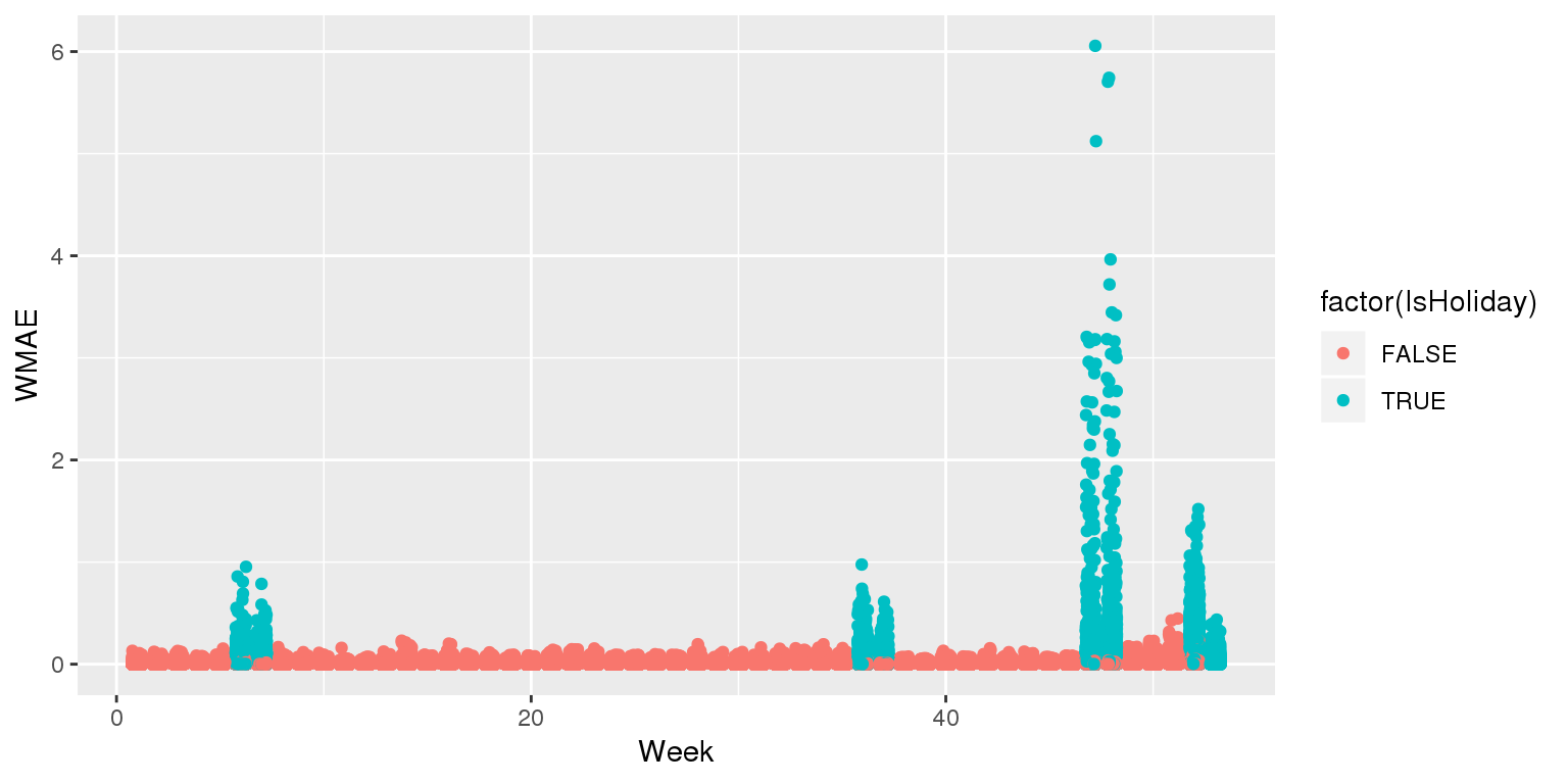
Visualizing in sample WMAE by Store
ggplot(data=df, aes(y=wmae_obs(actual=df$Weekly_Sales, predicted=df$WS_linear2,
                               holidays=df$IsHoliday),
                    x=week,
                    color=factor(Store))) +
  geom_jitter(width=0.25) + xlab("Week") + ylab("WMAE") +
  theme(legend.position="none")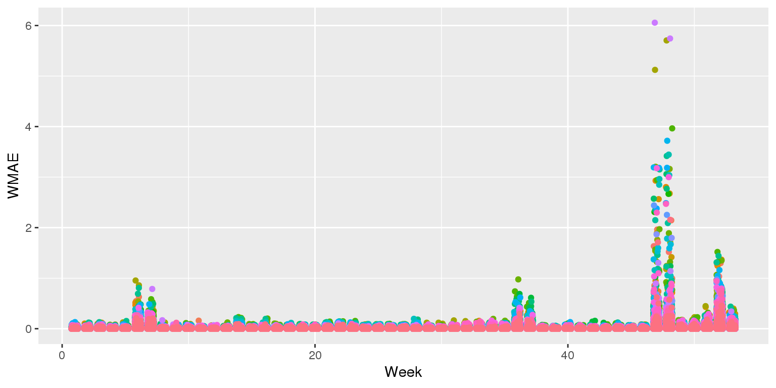
Visualizing in sample WMAE by Dept
ggplot(data=df, aes(y=wmae_obs(actual=df$Weekly_Sales, predicted=df$WS_linear2,
                               holidays=df$IsHoliday),
                    x=week,
                    color=factor(Dept))) +
  geom_jitter(width=0.25) + xlab("Week") + ylab("WMAE") +
  theme(legend.position="none")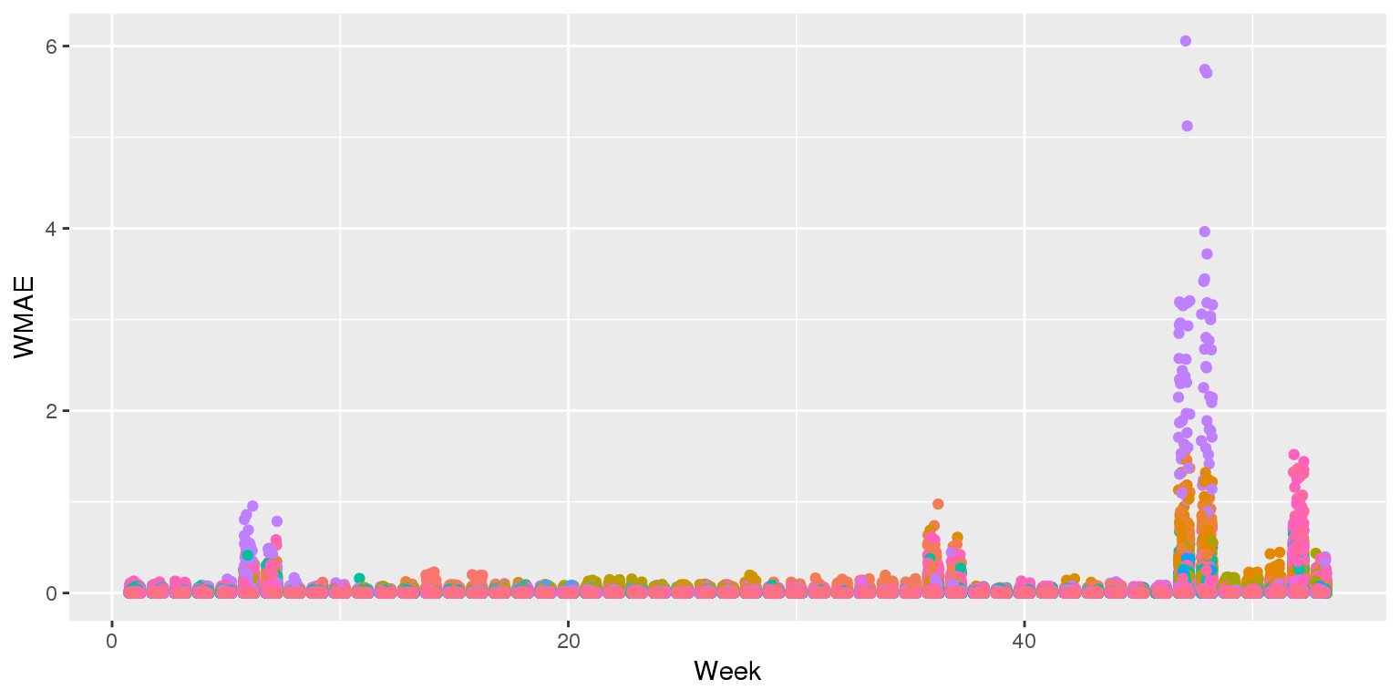
Back to the drawing board…
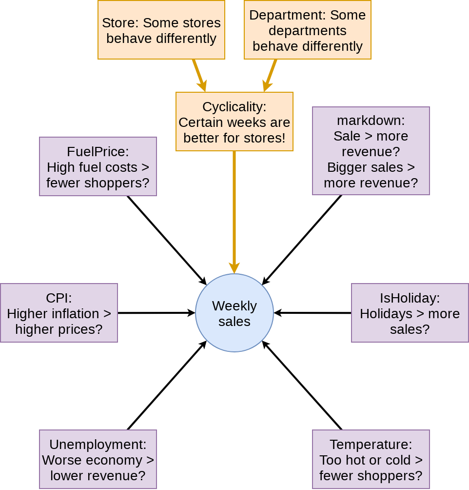
Third model: Including week x Store x Dept
mod3 <- lm(Weekly_mult ~ factor(week):factor(Store):factor(Dept) + factor(IsHoliday) + factor(markdown>0) +
                         markdown + Temperature +
                         Fuel_Price + CPI + Unemployment,
           data=df)
## Error: cannot allocate vector of size 606.8Gb
…
Third model: Including week x Store x Dept
library(lfe)
mod3 <- felm(Weekly_mult ~ markdown +
            Temperature +
            Fuel_Price +
            CPI +
            Unemployment | swd, data=df)
tidy(mod3)
## # A tibble: 5 x 5
## term estimate std.error statistic p.value
## <chr> <dbl> <dbl> <dbl> <dbl>
## 1 markdown -0.00000139 0.000000581 -2.40 1.65e- 2
## 2 Temperature 0.00135 0.000442 3.05 2.28e- 3
## 3 Fuel_Price -0.0637 0.00695 -9.17 4.89e-20
## 4 CPI 0.00150 0.00102 1.46 1.43e- 1
## 5 Unemployment -0.0303 0.00393 -7.70 1.32e-14glance(mod3)## # A tibble: 1 x 7
## r.squared adj.r.squared sigma statistic p.value df df.residual
## <dbl> <dbl> <dbl> <dbl> <dbl> <dbl> <dbl>
## 1 0.823 0.712 1.09 7.43 0 259457 259457PROBLEM
- We need to be able to predict out of sample to make our submission
felm() models don’t support predict
- So build it:
predict.felm <- function(object, newdata, use.fe=T, ...) {
  # compatible with tibbles
  newdata <- as.data.frame(newdata)
  co <- coef(object)

  y.pred <- t(as.matrix(unname(co))) %*% t(as.matrix(newdata[,names(co)]))

  fe.vars <- names(object$fe)

  all.fe <- getfe(object)
  for (fe.var in fe.vars) {
    level <- all.fe[all.fe$fe == fe.var,]
    frows <- match(newdata[[fe.var]],level$idx)
    myfe <- level$effect[frows]
    myfe[is.na(myfe)] = 0

    y.pred <- y.pred + myfe
  }
  as.vector(y.pred)
}
Prep submission and check in sample WMAE
# Out of sample result
df_test$Weekly_mult <- predict(mod3, df_test)
df_test$Weekly_Sales <- df_test$Weekly_mult * df_test$store_avg

# Required to submit a csv of Id and Weekly_Sales
write.csv(df_test[,c("Id","Weekly_Sales")],
          "WMT_FE.csv",
          row.names=FALSE)

# track
df_test$WS_FE <- df_test$Weekly_Sales

# Check in sample WMAE
df$WS_FE <- predict(mod3, df) * df$store_avg
w <- wmae(actual=df$Weekly_Sales, predicted=df$WS_FE, holidays=df$IsHoliday)
names(w) <- "FE"
wmaes <- c(wmaes, w)
wmaes
## Linear Linear 2 FE
## 3073.570 3230.643 1552.173Visualizing in sample WMAE
df$wmaes  <- wmae_obs(actual=df$Weekly_Sales, predicted=df$WS_FE,
                      holidays=df$IsHoliday)
ggplot(data=df, aes(y=wmaes,
                    x=week,
                    color=factor(IsHoliday))) +
  geom_jitter(width=0.25) + xlab("Week") + ylab("WMAE")
Maybe the data is part of the problem?
- What problems might there be for our testing sample?
- What is different from testing to training?
- Can we fix them?
- If so, how?
This was a real problem!
- Walmart provided this data back in 2014 as part of a recruiting exercise
- This is what the group project will be like
- 4 to 5 group members tackling a real life data problem
- You will have training data but testing data will be withheld
- Submit on Kaggle
Project deliverables
- Kaggle submission
- Your code for your submission, walking through what you did
- A 15 minute presentation on the last day of class describing:
- Your approach
- A report discussing
- Main points and findings
- Exploratory analysis of the data used
- Your model development, selection, implementation, evaluation, and refinement
- A conclusion on how well your group did and what you learned in the process
Binary outcomes
What are binary outcomes?
- Thus far we have talked about events with continuous outcomes
- Revenue: Some positive number
- Earnings: Some number
- ROA: Some percentage
- Binary outcomes only have two possible outcomes
- Did something happen, yes or no?
- Is a statement true or false?
Accounting examples of binary outcomes
- Financial:
- Will the company’s earnings meet analysts’ expectations
- Will the company have positive earnings?
- Managerial:
- Will we have ___ problem with our supply chain?
- Will our customer go bankrupt?
- Audit:
- Is the company committing fraud?
- Tax:
- Is the company too aggressive in their tax positions
We can assign a probability to any of these
Regression approach: Logistic regression
- When approaching a binary outcome, we use a logistic regression
- A.k.a. logit model
- The logit function is logit(x) = \text{log}\left(\frac{x}{1-x}\right)
- Also called log odds
\text{log}\left(\frac{\text{Prob}(y=1|X)}{1-\text{Prob}(y=1|X)}\right)=\alpha + \beta_1 x_1 + \beta_2 x_2 + \ldots + \varepsilon
Implementation: Logistic regression
- The logistic model is related to our previous linear models as such:
Both linear and logit models are under the class of General Linear Models (GLMs)
- To regress a GLM, we use the glm() command.
- To run a Logit regression:
mod <- glm(y ~ x1 + x2 + x3 + ..., data=df, family=binomial)

summary(mod)
Interpreting logit values
- The sign of the coefficients means the same as before
- +: increases the likelihood of y occurring
- -: decreases the likelihood of y occurring
- The level of the coefficient is different
- The relationship isn’t linear between x_i and y now
- Instead, coefficient is in log odds
- Thus, e^{\beta_i} gives you the odds, o
- To get probability, p, we can calculate p=\frac{o}{1+o}
- You can directly interpret the log odds for a coefficient (increased by \beta\%)
- You can directly interpret the odds for a coefficient (increased by (o-1)\%)
- You need to sum all relevant log odds before converting to probability!
Odds vs probability
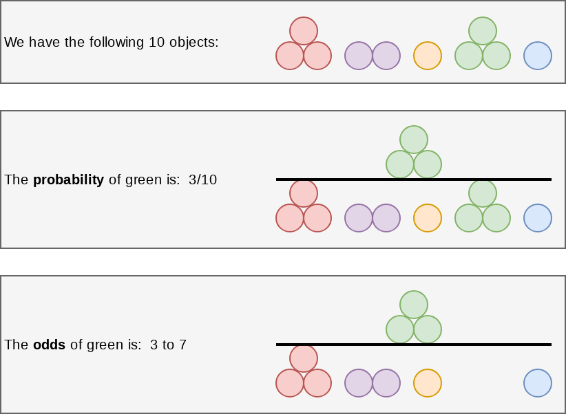
Example logit regression
Do holidays increase the likelihood that a department more than doubles its store’s average weekly sales across departments?
# Create the binary variable
df$double <- ifelse(df$Weekly_Sales > df$store_avg*2,1,0)
fit <- glm(double ~ IsHoliday, data=df, family=binomial)
summary(fit)##
## Call:
## glm(formula = double ~ IsHoliday, family = binomial, data = df)
##
## Deviance Residuals:
## Min 1Q Median 3Q Max
## -0.3260 -0.2504 -0.2504 -0.2504 2.6375
##
## Coefficients:
## Estimate Std. Error z value Pr(>|z|)
## (Intercept) -3.446804 0.009236 -373.19 <2e-16 ***
## IsHolidayTRUE 0.538640 0.027791 19.38 <2e-16 ***
## ---
## Signif. codes: 0 '***' 0.001 '**' 0.01 '*' 0.05 '.' 0.1 ' ' 1
##
## (Dispersion parameter for binomial family taken to be 1)
##
## Null deviance: 120370 on 421569 degrees of freedom
## Residual deviance: 120039 on 421568 degrees of freedom
## AIC: 120043
##
## Number of Fisher Scoring iterations: 6Converting logit coefficients
odds <- exp(coef(fit))
odds
## (Intercept) IsHolidayTRUE
## 0.03184725 1.71367497probability <- odds / (1 + odds)
probability## (Intercept) IsHolidayTRUE
## 0.03086431 0.63149603R practice: Logit
- A continuation of last week’s practices answering:
- Is Walmart more likely to see a year over year decrease in quarterly revenue during a recession?
- Practice using mutate() and glm()
- Do exercises 1 and 2 in today’s practice file
- R Practice
- Shortlink: rmc.link/420r5
Today’s Application: Shipping delays
The question
Can we leverage global weather data to predict shipping delays?

A bit about shipping data
- WRDS doesn’t have shipping data
- There are, however, vendors for shipping data, such as:
- They pretty much have any data you could need:
- Over 650,000 ships tracked using ground and satellite based AIS
- AIS: Automatic Identification System
- Live mapping
- Weather data
- Fleet tracking
- Port congestion
- Inmarsat support for ship operators
- Over 650,000 ships tracked using ground and satellite based AIS
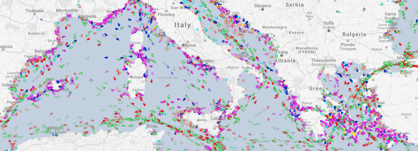
What can we see from naval data?
Yachts in the Mediterranean
Oil tankers in the Persian gulf

What can we see from naval data?
Shipping route via the Panama canal
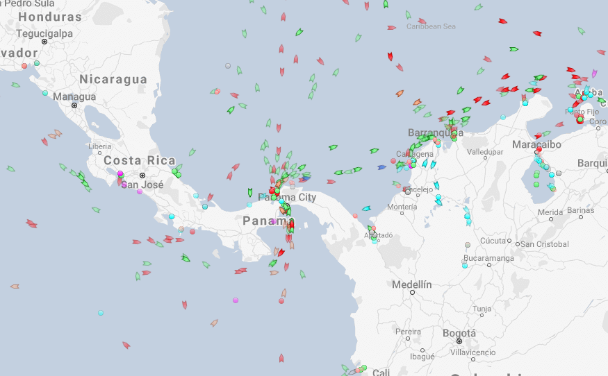
River shipping on the Mississippi river, USA
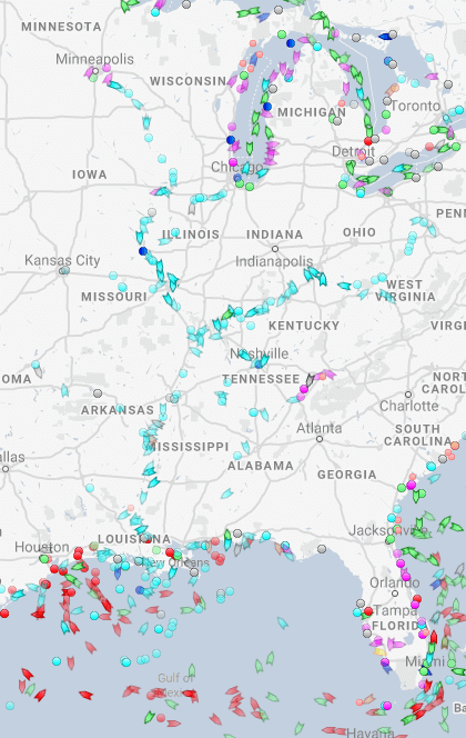
What can we see from naval data?
Busiest ports by containers and tons (Shanghai & Ningbo-Zhoushan, China) 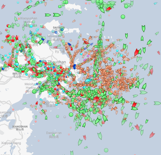
Busiest port for transshipment (Singapore)

Examining Singaporean owned ships
Code for last slide’s map
library(plotly)  # for plotting
library(RColorBrewer)  # for colors
# plot with boats, ports, and typhoons
# Note: geo is defined in the appendix -- it controls layout
palette = brewer.pal(8, "Dark2")[c(1,8,3,2)]
p <- plot_geo(colors=palette) %>%
  add_markers(data=df_ports, x = ~port_lon, y = ~port_lat, color = "Port") %>%
  add_markers(data=df_Aug31, x = ~lon, y = ~lat, color = ~ship_type,
              text=~paste('Ship name',shipname)) %>%
  add_markers(data=typhoon_Aug31, x = ~lon, y = ~lat, color="TYPHOON",
              text=~paste("Name", typhoon_name)) %>%
   layout(showlegend = TRUE, geo = geo,
    title = 'Singaporean owned container and tanker ships, August 31, 2018')
p- plot_geo() is from plotly
- add_markers() adds points to the map
- layout() adjusts the layout
- Within geo, a list, the following makes the map a globe
projection=list(type="orthographic")
Singaporean ship movement
Code for last slide’s map
library(sf)  # Note: very difficult to install except on Windows
library(maps)
# Requires separately installing "maptools" and "rgeos" as well
# This graph requires ~7GB of RAM to render
world1 <- sf::st_as_sf(map('world', plot = FALSE, fill = TRUE))

df_all <- df_all %>% arrange(run, imo)

p <- ggplot(data = world1) +
  geom_sf() +
  geom_point(data = df_all, aes(x = lon, y = lat, frame=frame,
                                text=paste("name:",shipname)))
ggplotly(p) %>%
   animation_opts(
1000, easing = "linear", redraw = FALSE)world1contains the map data- geom_sf() plots map data passed to ggplot()
- geom_point() plots ship locations as longitude and latitude
- ggplotly() converts the graph to html and animates it
- Animation follows the
frameaesthetic
- Animation follows the
What might matter for shipping?
What observable events or data might provide insight as to whether a naval shipment will be delayed or not?
Typhoon Jebi
Typhoons in the data
Code for last slide’s map
# plot with boats and typhoons
palette = brewer.pal(8, "Dark2")[c(1,3,2)]
p <- plot_geo(colors=palette) %>%
  add_markers(data=df_all[df_all$frame == 14,], x = ~lon, y = ~lat,
              color = ~ship_type, text=~paste('Ship name',shipname)) %>%
  add_markers(data=typhoon_Jebi, x = ~lon,
              y = ~lat, color="Typhoon Jebi",
              text=~paste("Name", typhoon_name, "</br>Time: ", date)) %>%
   layout(showlegend = TRUE, geo = geo,
    title = 'Singaporean container/tanker ships, September 4, 2018, evening')
p- This map is made the same way as the first map
Typhoons in the data using leaflet
Code for last slide’s map
library(leaflet)
library(leaflet.extras)
# icons
typhoonicons <- pulseIcons(color='red',
  heartbeat = ifelse(typhoon_Jebi$intensity_vmax > 150/1.852, 0.8,
    ifelse(typhoon$intensity_vmax < 118, 1.6, 1.2)),
  iconSize=ifelse(typhoon_Jebi$intensity_vmax > 150/1.852, 12,
    ifelse(typhoon_Jebi$intensity_vmax < 118, 3, 8)))
shipicons <- iconList(
  ship = makeIcon("../Figures/ship.png", NULL, 18, 18))
# plot
leaflet() %>%
  addTiles() %>%
  setView(lng = 136, lat = 34, zoom=4) %>%
  addPulseMarkers(data=typhoon_Jebi, lng=~lon, lat=~lat, label=~date,
                  icon=typhoonicons) %>%
  addMarkers(data=df_all[df_all$frame == 14,], lng=~lon, lat=~lat,
label=~shipname, icon=shipicons)- pulseIcons(): pulsing icons from leaflet.extras
- iconList(): pulls icons stored on your computer
- leaflet(): start the map; addTiles() pulls from OpenStreetMap
- setView(): sets the frame for the map
- addPulseMarkers(): adds pulsing markers
- addMarkers(): adds normal markers
R Practice on mapping
- Practice mapping typhoon data
- Practice using plotly and leaflet
- Do exercises 3 and 4 in today’s practice file
- R Practice
- Shortlink: rmc.link/420r5
Predicting delays due to typhoons
Data
- If the ship will report a delay of at least 3 hours in the next 12-24 hours
- Ship location
- Typhoon location
- Typhoon wind speed
We need to calculate distance between ships and typhoons
Distance for geo
- There are a number of formulas for this
- Haversine for a simple calculation
- Vincenty’s formulae for a complex, incredibly accurate calculation
- Accurate within 0.5mm
- Use distVincentyEllipsoid() from geosphere to get a reasonably quick and accurate calculation
- Calculates distance between two sets of points, x and y, structured as matrices
- Matrices must have longitude in the first column and latitude in the second column
- Provides distance in meters by default
library(geosphere)
x <- as.matrix(df3[,c("lon","lat")])  # ship location
y <- as.matrix(df3[,c("ty_lon","ty_lat")]) # typhoon location

df3$dist_typhoon <- distVincentyEllipsoid(x, y) / 1000
Clean up
- Some indicators to cleanly capture how far away the typhoon is
df3$typhoon_500 = ifelse(df3$dist_typhoon < 500 &
                         df3$dist_typhoon >= 0, 1, 0)
df3$typhoon_1000 = ifelse(df3$dist_typhoon < 1000 &
                          df3$dist_typhoon >= 500, 1, 0)
df3$typhoon_2000 = ifelse(df3$dist_typhoon < 2000 &
                          df3$dist_typhoon >= 1000, 1, 0)
Do typhoons delay shipments?
fit1 <- glm(delayed ~ typhoon_500 + typhoon_1000 + typhoon_2000, data=df3,
            family=binomial)
summary(fit1)
##
## Call:
## glm(formula = delayed ~ typhoon_500 + typhoon_1000 + typhoon_2000,
## family = binomial, data = df3)
##
## Deviance Residuals:
## Min 1Q Median 3Q Max
## -0.2502 -0.2261 -0.2261 -0.2261 2.7127
##
## Coefficients:
## Estimate Std. Error z value Pr(>|z|)
## (Intercept) -3.65377 0.02934 -124.547 <2e-16 ***
## typhoon_500 0.14073 0.16311 0.863 0.3883
## typhoon_1000 0.20539 0.12575 1.633 0.1024
## typhoon_2000 0.16059 0.07106 2.260 0.0238 *
## ---
## Signif. codes: 0 '***' 0.001 '**' 0.01 '*' 0.05 '.' 0.1 ' ' 1
##
## (Dispersion parameter for binomial family taken to be 1)
##
## Null deviance: 14329 on 59184 degrees of freedom
## Residual deviance: 14322 on 59181 degrees of freedom
## (3866 observations deleted due to missingness)
## AIC: 14330
##
## Number of Fisher Scoring iterations: 6It appears so!
Interpretation of coefficients
odds1 <- exp(coef(fit1))
odds1
## (Intercept) typhoon_500 typhoon_1000 typhoon_2000
## 0.02589334 1.15111673 1.22800815 1.17420736- Ships 1,000 to 2,000 km from a typhoon have 17% higher odds of having a delay
prob_odds1 <- c(exp(coef(fit1)[1]),
                exp(coef(fit1)[c(2, 3, 4)] + coef(fit1)[c(1, 1, 1)]))
probability1 <- prob_odds1 / (1 + prob_odds1)
probability1
## (Intercept) typhoon_500 typhoon_1000 typhoon_2000
## 0.02523980 0.02894356 0.03081733 0.02950702- Ships 1,000 to 2,000 km from a typhoon have a 3% chance of having a delay (baseline of 2.5%)
What about typhoon intensity?
- Hong Kong’s typhoon classification: Official source
- 41-62 km/h: Tropical depression
- 63-87 km/h: Tropical storm
- 88-117 km/h: Severe tropical storm
- 118-149 km/h: Typhoon
- 150-184 km/h: Severe typhoon
- 185+km/h: Super typhoon
# Cut makes a categorical variable out of a numerical variable using specified bins
df3$Super <- ifelse(df3$intensity_vmax * 1.852 > 185, 1, 0)
df3$Moderate <- ifelse(df3$intensity_vmax * 1.852 >= 88 &
                         df3$intensity_vmax * 1.852 < 185, 1, 0)
df3$Weak <- ifelse(df3$intensity_vmax * 1.852 >= 41 &
                   df3$intensity_vmax * 1.852 < 88, 1, 0)
df3$HK_intensity <- cut(df3$intensity_vmax ,c(41, 63, 88, 118, 150, 1000)/1.852)
table(df3$HK_intensity)
##
## (22.1,34] (34,47.5] (47.5,63.7] (63.7,81] (81,540]
## 13715 13228 9238 2255 21141Typhoon intensity and delays
fit2 <- glm(delayed ~ (typhoon_500 + typhoon_1000 + typhoon_2000) :
              (Weak + Moderate + Super), data=df3,
            family=binomial)
tidy(fit2)
## # A tibble: 10 x 5
## term estimate std.error statistic p.value
## <chr> <dbl> <dbl> <dbl> <dbl>
## 1 (Intercept) -3.65 0.0290 -126. 0
## 2 typhoon_500:Weak -0.00879 0.213 -0.0413 0.967
## 3 typhoon_500:Moderate 0.715 0.251 2.86 0.00430
## 4 typhoon_500:Super -8.91 123. -0.0726 0.942
## 5 typhoon_1000:Weak 0.250 0.161 1.55 0.121
## 6 typhoon_1000:Moderate 0.123 0.273 0.451 0.652
## 7 typhoon_1000:Super -0.0269 0.414 -0.0648 0.948
## 8 typhoon_2000:Weak 0.182 0.101 1.80 0.0723
## 9 typhoon_2000:Moderate 0.0253 0.134 0.189 0.850
## 10 typhoon_2000:Super 0.311 0.136 2.29 0.0217Moderate storms predict delays when within 500km
Super typhoons predict delays when 1,000 to 2,000km away
Interpretation of coefficients
odds2 <- exp(coef(fit2))
odds2[c(1, 3, 10)]
## (Intercept) typhoon_500:Moderate typhoon_2000:Super
## 0.02589637 2.04505487 1.36507575- Ships within 500km of a moderately strong storm have 104% higher odds of being delayed
- Ships 1,000 to 2,000km from a super typhoon have 36% higher odds
prob_odds2 <- c(exp(coef(fit2)[1]),
                exp(coef(fit2)[c(3, 10)] + coef(fit2)[c(1, 1)]))
probability2 <- prob_odds2 / (1 + prob_odds2)
probability2
## (Intercept) typhoon_500:Moderate typhoon_2000:Super
## 0.02524268 0.05029586 0.03414352- Ships within 500km of a moderately strong storm have a 5% chance of being delayed (baseline: 2.5%)
- Ships 1,000 to 2,000km from a super typhoon have a 3.4% chance
What might matter for shipping?
What other observable events or data might provide insight as to whether a naval shipment will be delayed or not?
- What is the reason that this event or data would be useful in predicting delays?
- I.e., how does it fit into your mental model?
End matter
For next week
- For next week:
- Second individual assignment
- Finish by the end of next Thursday
- Submit on eLearn
- Think about who you want to work with for the project
- Second individual assignment
Packages used for these slides
Custom code
# styling for plotly maps
geo <- list(
  showland = TRUE,
  showlakes = TRUE,
  showcountries = TRUE,
  showocean = TRUE,
  countrywidth = 0.5,
  landcolor = toRGB("grey90"),
  lakecolor = toRGB("aliceblue"),
  oceancolor = toRGB("aliceblue"),
  projection = list(
    type = 'orthographic',  # detailed at https://plot.ly/r/reference/#layout-geo-projection
    rotation = list(
      lon = 100,
      lat = 1,
      roll = 0
    )
  ),
  lonaxis = list(
    showgrid = TRUE,
    gridcolor = toRGB("gray40"),
    gridwidth = 0.5
  ),
  lataxis = list(
    showgrid = TRUE,
    gridcolor = toRGB("gray40"),
    gridwidth = 0.5
  )
)