ACCT 420: Logistic Regression for Bankruptcy


Session 6


Dr. Richard M. Crowley

Front matter

Learning objectives

  • Theory:
    • Academic research
  • Application:
    • Predicting bankruptcy over the next year for US manufacturing firms
      • Extend to credit downgrades
  • Methodology:
    • Logistic regression
    • Models from academic research

Datacamp

  • Explore on your own
  • No specific required class this week

Final exam expectations

  • 2 hour exam (planned)
  • Multiple choice (~30%)
    • Focused on coding
  • Long format (~70%), possible questions:
    • Propose and explain a model to solve a problem
    • Explain the implementation of a model
    • Interpret results
    • Propose visualizations to illustrate a result
    • Interpret visualizations

Group project

Possible competition choices:

  1. Deciding to extend (or not extend) loans to those with no banking history
  2. Predicting a Google Store’s revenue
  3. Forecasting the number of followers companies had on Twitter in 2017
  4. Detecting restatements caused by intentional misrepresentation by managers in the US

5 per group. Sign up at rmc.link/420groups

Logistic regression interpretation

A simple interpretation

  • Last week we had the model:

logodds(Double~sales) = -3.44 + 0.54 Holiday

  • There are two ways to interpret this:
    1. Coefficient by coefficient
    2. In total

Interpretting specific coefficients

logodds(Double~sales) = -3.44 + 0.54 Holiday

  • Interpreting specific coefficients is easiest done manually
    • Odds for Holiday are exp(0.54) = 1.72
      • This means that having a holiday modifies the baseline (i.e., non-Holiday) odds by 1.72 to 1
        • Where 1 to 1 is considered no change
    • Probability for Holiday is 1.72 / (1 + 1.72) = 0.63
      • This means that having a holiday modifies the baseline (i.e., non-Holiday) probability by 63%
        • Where 50% is considered no change

Interpretting in total

  • It is important to note that log odds are additive
    • So, calculate a new log odd by plugging in values for variables and adding it all up
      • Holiday: -3.44 + 0.54 * 1 = -2.9
      • No holiday: -3.44 + 0.54 * 0 = -3.44
  • Then calculate odds and log odds like before

Using predict() to simplify it

  • predict() can calculate log odds and probabilities for us with minimal effort
    • Specify type="response" to get probabilities
test_data <- as.data.frame(IsHoliday = c(0,1))
predict(model, test_data)  # log odds
## [1] -3.44 -2.90
predict(model, test_data, type="response")  #probabilities
## [1] 0.03106848 0.05215356
  • Here, we see the baseline probability is 3.1%
  • The probability of doubling sales on a holiday is higher, at 5.2%

These are a lot easier to interpret

Academic research

History of academic research in accounting

  • Academic research in accounting, as it is today, began in the 1960s
    • What we call Positive Accounting Theory
      • Positive theory: understanding how the world works
  • Prior to the 1960s, the focus was on Prescriptive theory
    • How the world should work
  • Accounting research builds on work from many fields:
    • Economics
    • Finance
    • Psychology
    • Econometrics
    • Computer science (more recently)

Types of academic research

  • Theory
    • Pure economics proofs and simulation
  • Experimental
    • Proper experimentation done on individuals
    • Can be psychology experiments or economic experiments
  • Empirical/Archival
    • Data driven research
    • Based on the usage of historical data (i.e., archives)
    • Most likely to be easily co-optable by businesses and regulators

Who leverages accounting research

  • Hedge funds
  • Mutual funds
  • Auditors
  • Law firms

Where can you find academic research

Academic models: Altman Z-Score

Where does the model come from?

  • Altman 1968, Journal of Finance
  • A seminal paper in Finance cited over 15,000 times by other academic papers

What is the model about?

  • The model was developed to identify firms likely to go bankrupt from a pool of firms
  • Focuses on using ratio analysis to determine such firms

Model specification

Z = 1.2 x_1 + 1.4 x_2 + 3.3 x_3 + 0.6 x_4 + 0.999 x_5

  • x_1: Working capital to assets ratio
  • x_2: Retained earnings to assets ratio
  • x_3: EBIT to assets ratio
  • x_4: Market value of equity to book value of liabilities
  • x_5: Sales to total assets

This looks like a linear regression without a constant

How did the measure come to be?

  • It actually isn’t a linear regression
    • It is a clustering method called MDA (multiple discriminant analysis)
      • There are newer methods these days, such as SVM
  • Used data from 1946 through 1965
    • 33 US manufacturing firms that went bankrupt, 33 that survived

More about this, from Altman himself in 2000: rmc.link/420class6

  • Read the section “Variable Selection” starting on page 8
    • Skim through x_1, x_2, x_3, x_4, and x_5 if you are interested in the ratios

How would these assumptions stand today?

Who uses it?

  • Despite the model’s simplicity and age, it is still in use
    • The simplicity of it plays a large part
  • Frequently used by financial analysts

Recent news mentioning it

Application

Main question

Can we use bankruptcy models to predict supplier bankruptcies?

But first:

Does the Altman Z-score [still] pick up bankruptcy?

Question structure

Is this a forecasting or forensics question?

  • It has a time dimension like a forecasting question
  • It has a feeling of a forensics question

The data

  • Compustat provides data on bankruptcies, including the date a company went bankrupt
    • Bankruptcy information is included in the “footnote” items in Compustat
      • If dlsrn == 2, then the firm went bankrupt
      • Bankruptcy date is dldte
  • All components of the Altman Z-Score model are in Compustat
    • But we’ll pull market value from CRSP, since it is more complete
  • All components of our later models are from Compustat as well
  • Company credit rating data also from Compustat (Rankings)

Bankruptcy in the US

  • Chapter 7
    • The company ceases operating and liquidates
  • Chapter 11
    • For firms intending to reorganize the company to “try to become profitable again” (US SEC)

Common outcomes of bankruptcy

  1. Cease operations entirely (liquidated)
    • In which case the assets are often sold off
  2. Acquired by another company
  3. Merge with another company
  4. Successfully restructure and continue operating as the same firm
  5. Restructure and operate as a new firm

Calculating bankruptcy

# initial cleaning
df <- df %>% filter(at >= 1, revt >= 1, gvkey != 100338)

## Merge in stock value
df$date <- as.Date(df$datadate)
df_mve$date <- as.Date(df_mve$datadate)
df_mve <- df_mve %>% rename(gvkey=GVKEY)
df_mve$MVE <- df_mve$csho * df_mve$prcc_f

df <- left_join(df, df_mve[,c("gvkey","date","MVE")])
## Joining, by = c("gvkey", "date")
df <- df %>%
  group_by(gvkey) %>%
  mutate(bankrupt = ifelse(row_number() == n() & dlrsn == 2 &
                           !is.na(dlrsn), 1, 0)) %>%
  ungroup()
  • row_number() gives the current row within the group, with the first row as 1, next as 2, etc.
  • n() gives the number of rows in the group

Calculating the Altman Z-Score

# Calculate the measures needed
df <- df %>%
  mutate(wcap_at = wcap / at,  # x1
         re_at = re / at,  # x2
         ebit_at = ebit / at,  # x3
         mve_lt = MVE / lt,  # x4
         revt_at = revt / at)  # x5
# cleanup
df <- df %>%
  mutate_if(is.numeric, funs(replace(., !is.finite(.), NA)))

# Calculate the score
df <- df %>%
  mutate(Z = 1.2 * wcap_at + 1.4 * re_at + 3.3 * ebit_at + 0.6 * mve_lt + 
           0.999 * revt_at)

# Calculate date info for merging
df$date <- as.Date(df$datadate)
df$year <- year(df$date)
df$month <- month(df$date)
  • Calculate x_1 through x_5
  • Apply the model directly

Build in credit ratings

We’ll check our Z-score against credit rating as a simple validation

# df_ratings has ratings data in it

# Ratings, in order from worst to best
ratings <- c("D", "C", "CC", "CCC-", "CCC","CCC+", "B-", "B", "B+", "BB-",
             "BB", "BB+", "BBB-", "BBB", "BBB+", "A-", "A", "A+", "AA-", "AA",
             "AA+", "AAA-", "AAA", "AAA+")
# Convert string ratings (splticrm) to numeric ratings
df_ratings$rating <- factor(df_ratings$splticrm, levels=ratings, ordered=T)

df_ratings$date <- as.Date(df_ratings$datadate)
df_ratings$year <- year(df_ratings$date)
df_ratings$month <- month(df_ratings$date)

# Merge together data
df <- left_join(df, df_ratings[,c("gvkey", "year", "month", "rating")])
## Joining, by = c("gvkey", "year", "month")

Z vs credit ratings, 1973-2017

df %>%
  filter(!is.na(Z),
         !is.na(bankrupt)) %>%
  group_by(bankrupt) %>%
  mutate(mean_Z=mean(Z,na.rm=T)) %>%
  slice(1) %>%
  ungroup() %>%
  select(bankrupt, mean_Z) %>%
  html_df()
bankrupt mean_Z
0 3.939223
1 0.927843

Z vs credit ratings, 2000-2017

df %>%
  filter(!is.na(Z),
         !is.na(bankrupt),
         year >= 2000) %>%
  group_by(bankrupt) %>%
  mutate(mean_Z=mean(Z,na.rm=T)) %>%
  slice(1) %>%
  ungroup() %>%
  select(bankrupt, mean_Z) %>%
  html_df()
bankrupt mean_Z
0 3.822281
1 1.417683

Test it with a regression

fit_Z <- glm(bankrupt ~ Z, data=df, family=binomial)
summary(fit_Z)
## 
## Call:
## glm(formula = bankrupt ~ Z, family = binomial, data = df)
## 
## Deviance Residuals: 
##     Min       1Q   Median       3Q      Max  
## -1.8297  -0.0676  -0.0654  -0.0624   3.7794  
## 
## Coefficients:
##             Estimate Std. Error z value Pr(>|z|)    
## (Intercept) -5.94354    0.11829 -50.245  < 2e-16 ***
## Z           -0.06383    0.01239  -5.151 2.59e-07 ***
## ---
## Signif. codes:  0 '***' 0.001 '**' 0.01 '*' 0.05 '.' 0.1 ' ' 1
## 
## (Dispersion parameter for binomial family taken to be 1)
## 
##     Null deviance: 1085.2  on 35296  degrees of freedom
## Residual deviance: 1066.5  on 35295  degrees of freedom
##   (15577 observations deleted due to missingness)
## AIC: 1070.5
## 
## Number of Fisher Scoring iterations: 9

So what?

  • Read this article: rmc.link/420class6-2
    • “Carillion’s liquidation reveals the dangers of shared sourcing”

Based on this article, why do we care about bankruptcy risk for other firms?

How good is the model though???

Examples:

Correct 92.0% of the time using Z < 1 as a cutoff

  • Correctly captures 39 of 83 bankruptcies

Correct 99.7% of the time if we say firms never go bankrupt…
  • Correctly captures 0 of 83 bankruptcies

Errors in binary testing

Types of errors

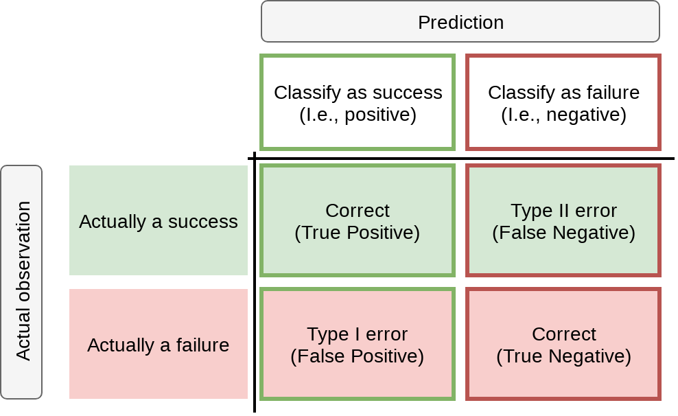
This type of chart (filled in) is called a Confusion matrix

Type I error (False positive)

We say that the company will go bankrupt, but they don’t

  • A Type I error occurs any time we say something is true, yet it is false
  • Quantifying type I errors in the data
    • False positive rate (FPR)
      • The percent of failures misclassified as successes
    • Specificity: 1 - FPR
      • A.k.a. true negative rate (TNR)
      • The percent of failures properly classified

Type 2 error (False negative)

We say that the company will not go bankrupt, yet they do

  • A Type II error occurs any time we say something is false, yet it is true
  • Quantifying type I errors in the data
    • False negative rate (FNR): 1-Sensitivity
      • The percent of successes misclassified as failures
    • Sensitivity:
      • A.k.a. true positive rate (TPR)
      • The percent of successes properly classified

Useful equations

A note on the equations

  • Accuracy is very useful if you are predicting something that occurs reasonably frequently
    • Not too often, but not too rarely
  • Sensitivity is very useful for rare events
  • Specificity is very useful for frequent events
    • Or for events where misclassifying the null is very troublesome
      • Criminal trials
      • Medical diagnoses

Let’s plot TPR and FPR out

  • ROCR can calculate these for us!
library(ROCR)
pred_Z <- predict(fit_Z, df, type="response")
ROCpred_Z <- prediction(as.numeric(pred_Z), as.numeric(df$bankrupt))
ROCperf_Z <- performance(ROCpred_Z, 'tpr','fpr')
  • Notes on ROCR:
    1. The functions are rather picky and fragile. Likely sources of error include:
      • The vectors passed to prediction() aren’t explicitly numeric
      • There are NAs in the data
    2. prediction() does not actually predict – it builds an object based on your prediction (first argument) and the actual outcomes (second argument)
    3. performance() calculates performance measures
      • It knows 30 of them
      • 'tpr' is true positive rate
      • 'fpr' is false positive rate

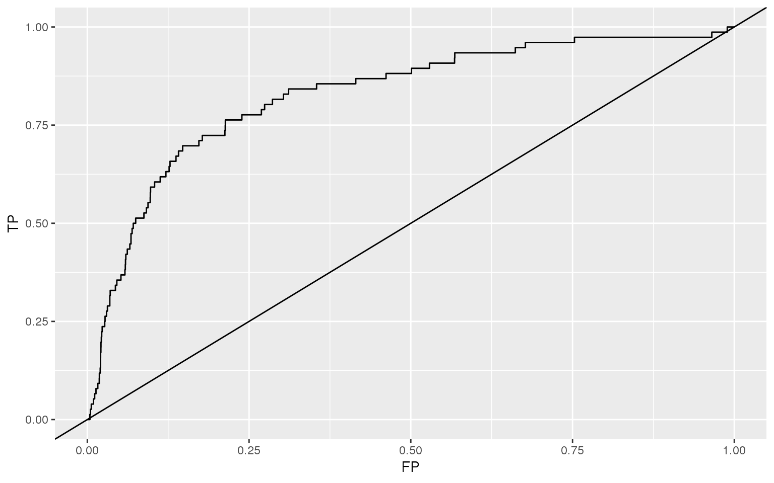
Let’s plot TPR and FPR out

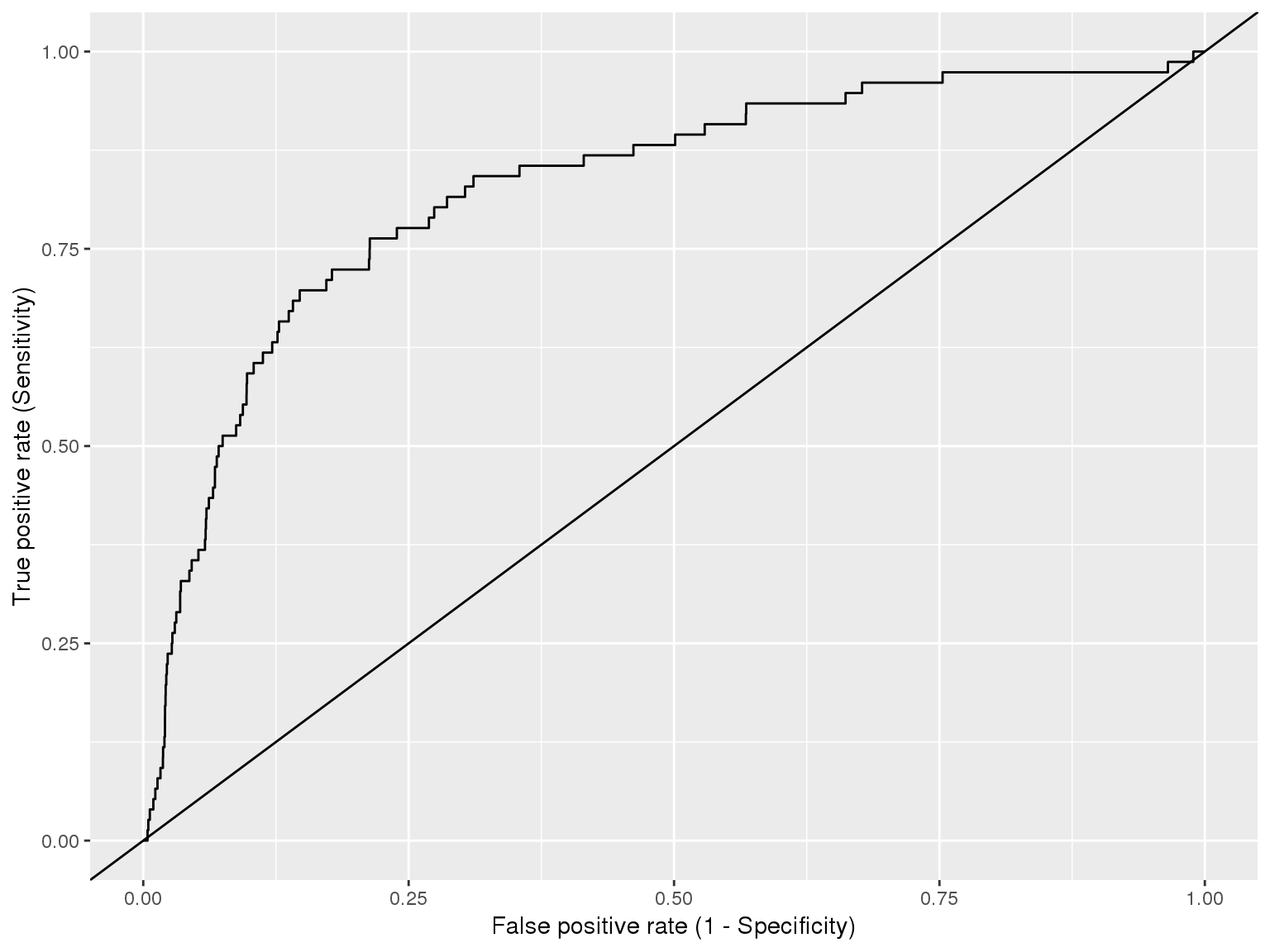
  • Two ways to plot it out:
df_ROC_Z <- data.frame(
  FP=c(ROCperf_Z@x.values[[1]]),
  TP=c(ROCperf_Z@y.values[[1]]))
ggplot(data=df_ROC_Z,
  aes(x=FP, y=TP)) + geom_line() +
  geom_abline(slope=1)
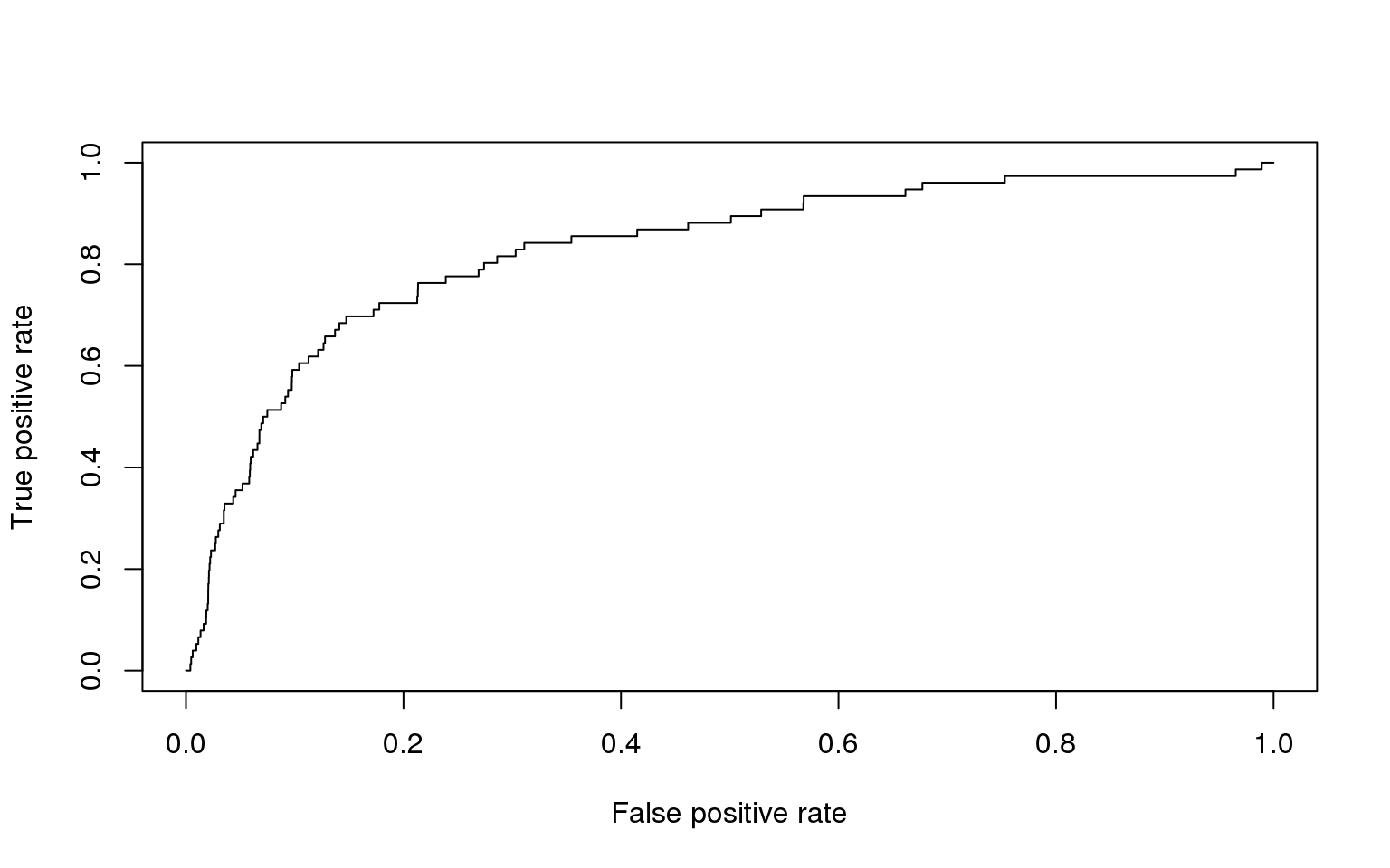
plot(ROCperf_Z)
ROC curves

  • The previous graph is called a ROC curve, or receiver operator characteristic curve
  • The higher up and left the curve is, the better the logistic regression fits.
  • Neat properties:
    • The area under a perfect model is always 1
    • The area under random chance is always 0.5

ROC AUC

  • The neat properties of the curve give rise to a useful statistic: ROC AUC
    • AUC = Area under the curve
  • Ranges from 0 (perfectly incorrect) to 1 (perfectly correct)
  • Above 0.6 is generally the minimum acceptable bound
    • 0.7 is preferred
    • 0.8 is very good
  • ROCR can calculate this too
auc_Z <- performance(ROCpred_Z, measure = "auc")
auc_Z@y.values[[1]]
## [1] 0.8280943
  • Note: The objects made by ROCR are not lists!
    • They are “S4 objects”
    • This is why we use @ to pull out values, not $
      • That’s the only difference you need to know here

R Practice ROC AUC

  • Practice using these new functions with last week’s Walmart data
    1. Model decreases in revenue using prior quarter YoY revenue growth
    2. Explore the model using predict()
    3. Calculate ROC AUC
    4. Plot an ROC curve
  • Do all exercises in today’s practice file

Academic models: Distance to default (DD)

Where does the model come from?

  • Merton 1974, Journal of Finance
  • Another seminal paper in finance, cited by over 12,000 other academic papers
  • About Merton

What is the model about?

  • The model itself comes from thinking of debt in an options pricing framework
  • Uses the Black-Scholes model to price out a company
  • Consider a company to be bankrupt when the company is not worth more than the the debt itself, in expectation

Model specification

DD = \frac{\log(V_A / D) + (r-\frac{1}{2}\sigma_A^2)(T-t)}{\sigma_A \sqrt(T-t)}
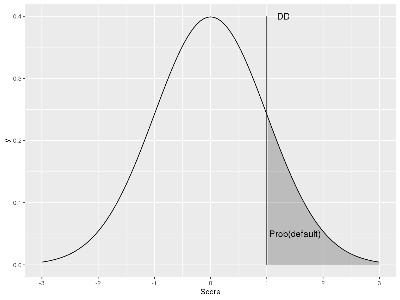
  • V_A: Value of assets
    • Market based
  • D: Value of liabilities
    • From balance sheet
  • r: The risk free rate
  • \sigma_A: Volatility of assets
    • Use daily stock return volatility, annualized
      • Annualized means multiply by \sqrt{252}
  • T-t: Time horizon

Who uses it?

  • Moody’s KMV is derived from the Merton model

Applying DD

Calculating DD in R

  • First we need one more measure: the standard deviation of assets
    • This varies by time, and construction of it is subjective
    • We will use standard deviation over the last 5 years
# df_stock is an already prepped csv from CRSP data
df_stock$date <- as.Date(df_stock$date)
df <- left_join(df, df_stock[,c("gvkey", "date", "ret", "ret.sd")])
## Joining, by = c("gvkey", "date")

Calculating DD in R

df_rf$date <- as.Date(df_rf$dateff)
df_rf$year <- year(df_rf$date)
df_rf$month <- month(df_rf$date)

df <- left_join(df, df_rf[,c("year", "month", "rf")])
## Joining, by = c("year", "month")
df <- df %>%
  mutate(DD = (log(MVE / lt) + (rf - (ret.sd*sqrt(252))^2 / 2)) /
              (ret.sd*sqrt(252)))
# Clean the measure
df <- df %>%
  mutate_if(is.numeric, funs(replace(., !is.finite(.), NA)))
  • Just apply the formula using mutate
  • \sqrt{252} is included because ret.sd is daily return standard deviation
    • There are ~252 trading days per year in the US

DD vs credit ratings, 1973-2017

df %>%
  filter(!is.na(DD),
         !is.na(bankrupt)) %>%
  group_by(bankrupt) %>%
  mutate(mean_DD=mean(DD, na.rm=T),
         prob_default =
           pnorm(-1 * mean_DD)) %>%
  slice(1) %>%
  ungroup() %>%
  select(bankrupt, mean_DD,
         prob_default) %>%
  html_df()
bankrupt mean_DD prob_default
0 0.612414 0.2701319
1 -2.447382 0.9928051

DD vs credit ratings, 2000-2017

df %>%
  filter(!is.na(DD),
         !is.na(bankrupt),
         year >= 2000) %>%
  group_by(bankrupt) %>%
  mutate(mean_DD=mean(DD, na.rm=T),
         prob_default =
           pnorm(-1 * mean_DD)) %>%
  slice(1) %>%
  ungroup() %>%
  select(bankrupt, mean_DD,
         prob_default) %>%
  html_df()
bankrupt mean_DD prob_default
0 0.8411654 0.2001276
1 -4.3076039 0.9999917

Test it with a regression

fit_DD <- glm(bankrupt ~ DD, data=df, family=binomial)
## Warning: glm.fit: fitted probabilities numerically 0 or 1 occurred
summary(fit_DD)
## 
## Call:
## glm(formula = bankrupt ~ DD, family = binomial, data = df)
## 
## Deviance Residuals: 
##     Min       1Q   Median       3Q      Max  
## -2.9848  -0.0750  -0.0634  -0.0506   3.6506  
## 
## Coefficients:
##             Estimate Std. Error z value Pr(>|z|)    
## (Intercept) -6.16401    0.15323  -40.23  < 2e-16 ***
## DD          -0.24451    0.03773   -6.48 9.14e-11 ***
## ---
## Signif. codes:  0 '***' 0.001 '**' 0.01 '*' 0.05 '.' 0.1 ' ' 1
## 
## (Dispersion parameter for binomial family taken to be 1)
## 
##     Null deviance: 718.67  on 21563  degrees of freedom
## Residual deviance: 677.18  on 21562  degrees of freedom
##   (33618 observations deleted due to missingness)
## AIC: 681.18
## 
## Number of Fisher Scoring iterations: 9

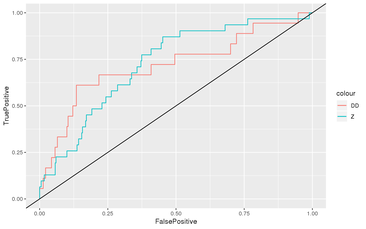
ROC Curves

pred_DD <- predict(fit_DD, df, type="response")
ROCpred_DD <- prediction(as.numeric(pred_DD), as.numeric(df$bankrupt))
ROCperf_DD <- performance(ROCpred_DD, 'tpr','fpr')
df_ROC_DD <- data.frame(FalsePositive=c(ROCperf_DD@x.values[[1]]),
                 TruePositive=c(ROCperf_DD@y.values[[1]]))
ggplot() +
  geom_line(data=df_ROC_DD, aes(x=FalsePositive, y=TruePositive, color="DD")) + 
  geom_line(data=df_ROC_Z, aes(x=FP, y=TP, color="Z")) + 
  geom_abline(slope=1)
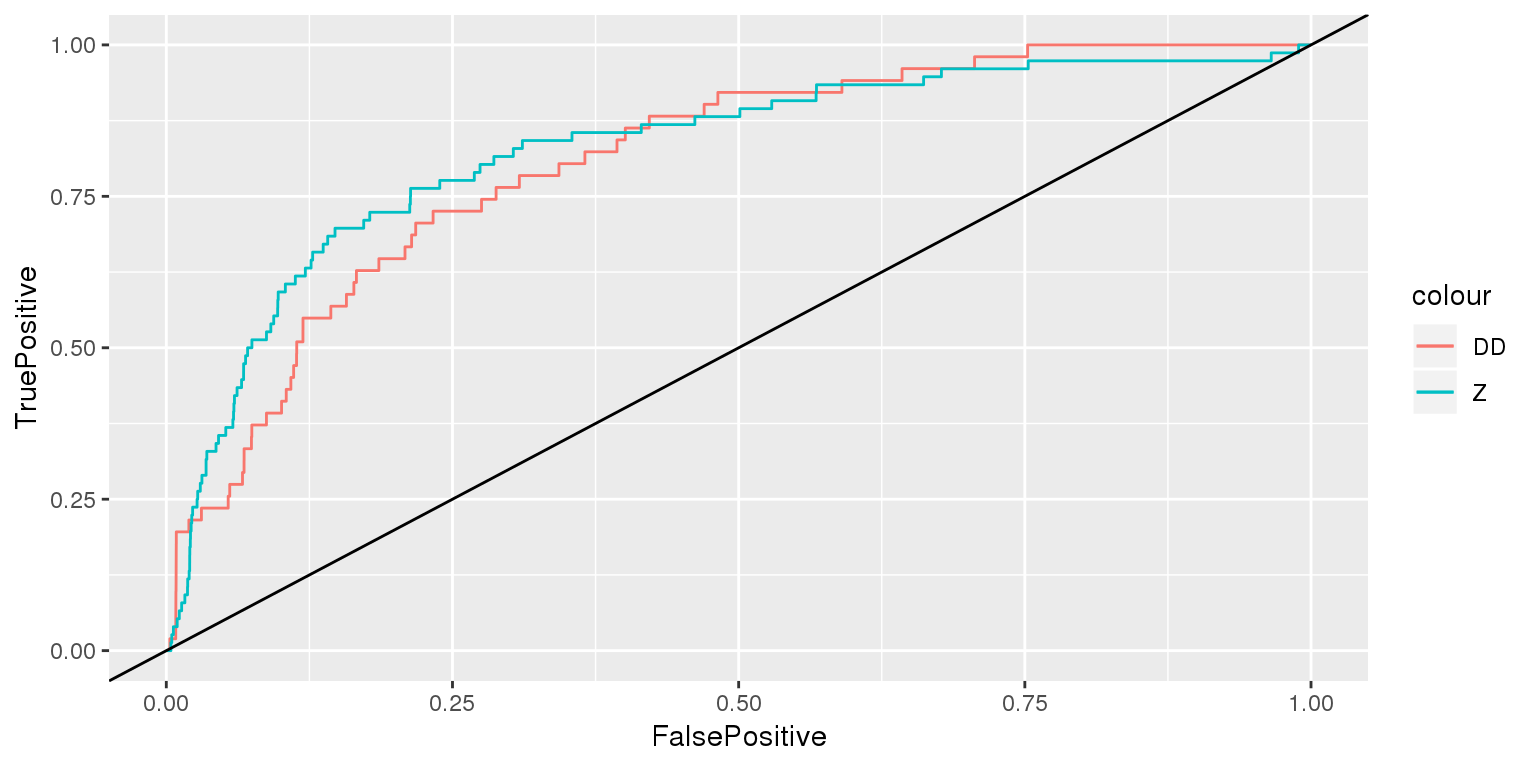
AUC comparison

#AUC
auc_DD <- performance(ROCpred_DD, measure = "auc")
AUCs <- c(auc_Z@y.values[[1]], auc_DD@y.values[[1]])
names(AUCs) <- c("Z", "DD")
AUCs
##         Z        DD 
## 0.8280943 0.8097803

Both measures perform similarly, but Altman Z performs slightly better.

A more practical application

A more practical application

  • Companies don’t only have problems when there is a bankruptcy
    • Credit downgrades can be just as bad

Why?

  • Credit downgrades cause an increase in interest rates for debt, leading to potential liquidity issues.

Predicting downgrades

# calculate downgrade
df <- df %>% arrange(gvkey, date) %>% group_by(gvkey) %>% mutate(downgrade = ifelse(rating < lag(rating),1,0))

# training sample
train <- df %>% filter(year < 2015)
test <- df %>% filter(year >= 2015)

# glms
fit_Z2 <- glm(downgrade ~ Z, data=train, family=binomial)
## Warning: glm.fit: fitted probabilities numerically 0 or 1 occurred
fit_DD2 <- glm(downgrade ~ DD, data=train, family=binomial)

Predicting downgrades with Altman Z

summary(fit_Z2)
## 
## Call:
## glm(formula = downgrade ~ Z, family = binomial, data = train)
## 
## Deviance Residuals: 
##     Min       1Q   Median       3Q      Max  
## -1.1223  -0.5156  -0.4418  -0.3277   6.4638  
## 
## Coefficients:
##             Estimate Std. Error z value Pr(>|z|)    
## (Intercept) -1.10377    0.09288  -11.88   <2e-16 ***
## Z           -0.43729    0.03839  -11.39   <2e-16 ***
## ---
## Signif. codes:  0 '***' 0.001 '**' 0.01 '*' 0.05 '.' 0.1 ' ' 1
## 
## (Dispersion parameter for binomial family taken to be 1)
## 
##     Null deviance: 3874.5  on 5795  degrees of freedom
## Residual deviance: 3720.4  on 5794  degrees of freedom
##   (47058 observations deleted due to missingness)
## AIC: 3724.4
## 
## Number of Fisher Scoring iterations: 6

Predicting downgrades with DD

summary(fit_DD2)
## 
## Call:
## glm(formula = downgrade ~ DD, family = binomial, data = train)
## 
## Deviance Residuals: 
##     Min       1Q   Median       3Q      Max  
## -1.7319  -0.5004  -0.4278  -0.3343   3.0755  
## 
## Coefficients:
##             Estimate Std. Error z value Pr(>|z|)    
## (Intercept) -2.36365    0.05607  -42.15   <2e-16 ***
## DD          -0.22224    0.02035  -10.92   <2e-16 ***
## ---
## Signif. codes:  0 '***' 0.001 '**' 0.01 '*' 0.05 '.' 0.1 ' ' 1
## 
## (Dispersion parameter for binomial family taken to be 1)
## 
##     Null deviance: 3115.3  on 4732  degrees of freedom
## Residual deviance: 2982.9  on 4731  degrees of freedom
##   (48121 observations deleted due to missingness)
## AIC: 2986.9
## 
## Number of Fisher Scoring iterations: 5
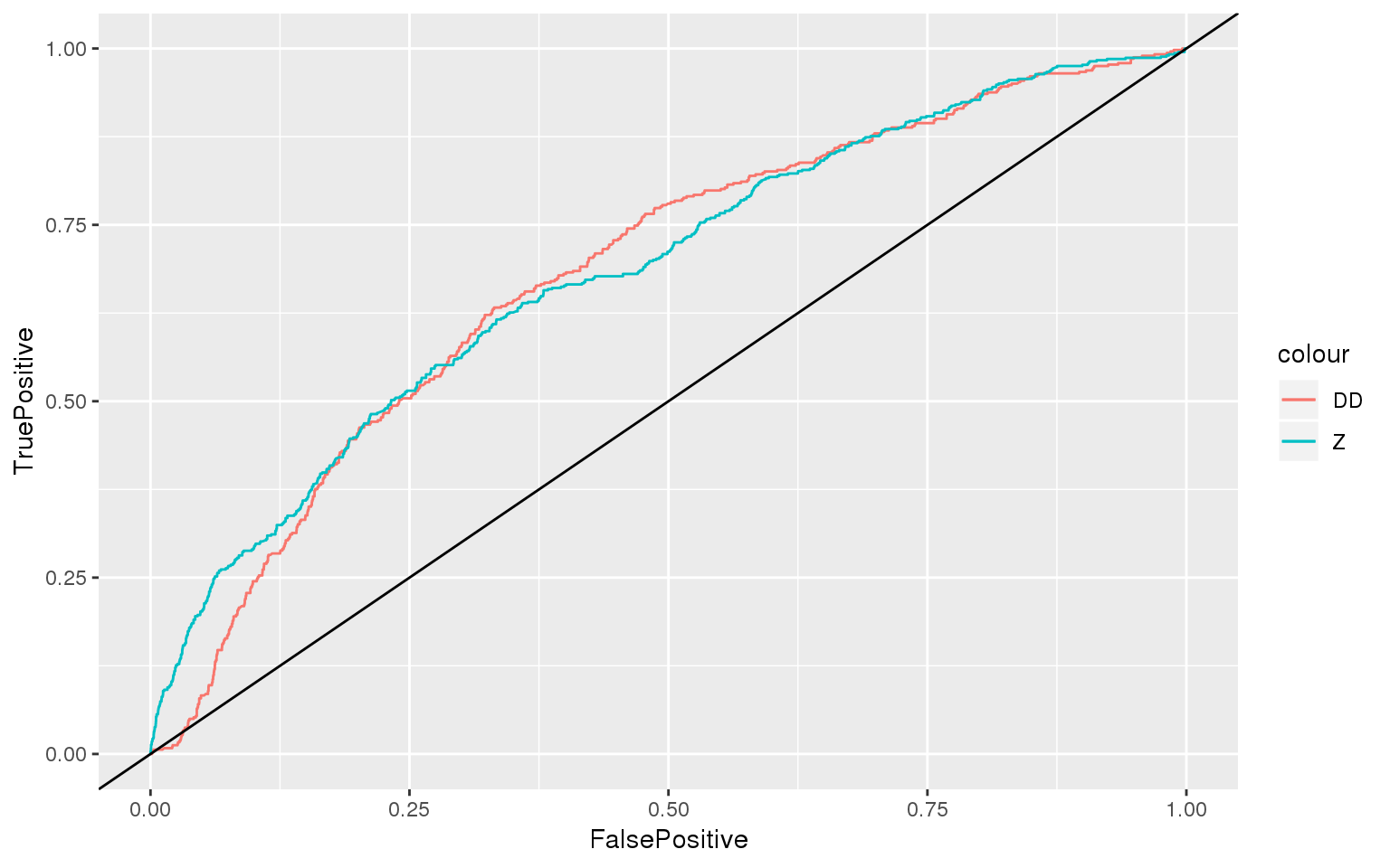
ROC Performance on this task

##         Z        DD 
## 0.6839086 0.6811973

Out of sample ROC performance

##         Z        DD 
## 0.7270046 0.7183575

Predicting bankruptcy

What other data could we use to predict corporate bankruptcy as it relates to a company’s supply chain?

  • What is the reason that this event or data would be useful for prediction?
    • I.e., how does it fit into your mental model?
  • A useful starting point from McKinsey

End matter

For next week

  • For next week:
    • Second individual assignment
      • Finish by the end of Thursday
      • Submit on eLearn
    • Datacamp
      • Practice a bit more to keep up to date
        • Using R more will make it more natural

Packages used for these slides

Custom code