ACCT 420: ML and AI for visual data
Session 11
Dr. Richard M. Crowley
Front matter
Learning objectives
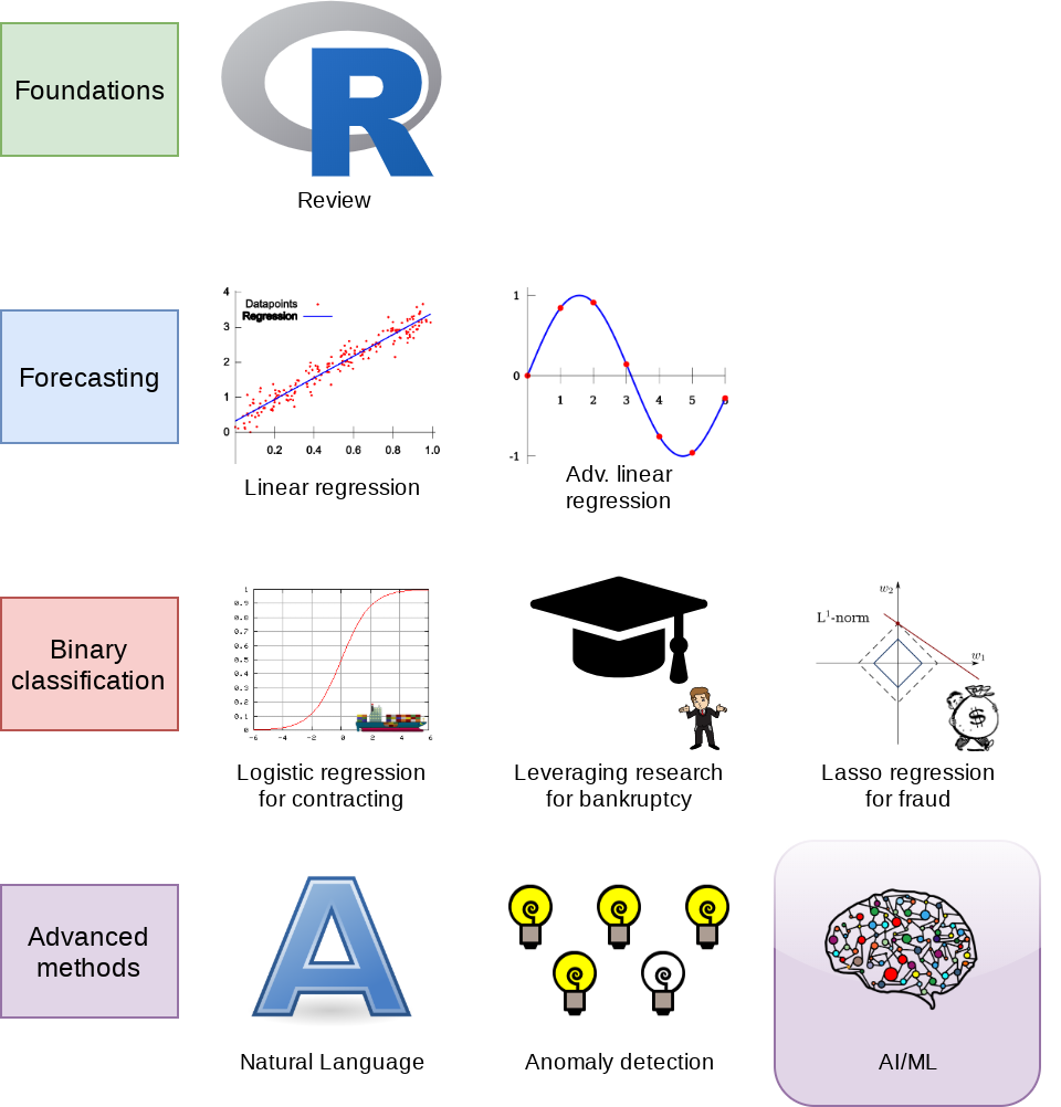
- Theory:
- Neural Networks for…
- Images
- Audio
- Video
- Neural Networks for…
- Application:
- Handwriting recognition
- Identifying financial information in images
- Methodology:
- Neural networks
- CNNs
- Neural networks
Group project
- Next class you will have an opportunity to present your work
- ~15 minutes per group
- You will also need to submit your report & code on Tuesday
- Please submit as a zip file
- Be sure to include your report AND code AND slides
- Code should cover your final model
- Covering more is fine though
- Code should cover your final model
- Competitions close Sunday night!
Image data
Thinking about images as data
- Images are data, but they are very unstructured
- No instructions to say what is in them
- No common grammar across images
- Many, many possible subjects, objects, styles, etc.
- From a computer’s perspective, images are just 3-dimensional matrices
- Rows (pixels)
- Columns (pixels)
- Color channels (usually Red, Green, and Blue)
Using images as data
- We can definitely use numeric matrices as data
- We did this plenty with XGBoost, for instance
- However, images have a lot of different numbers tied to each observation.
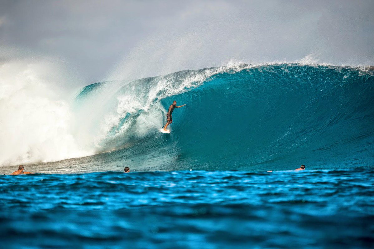
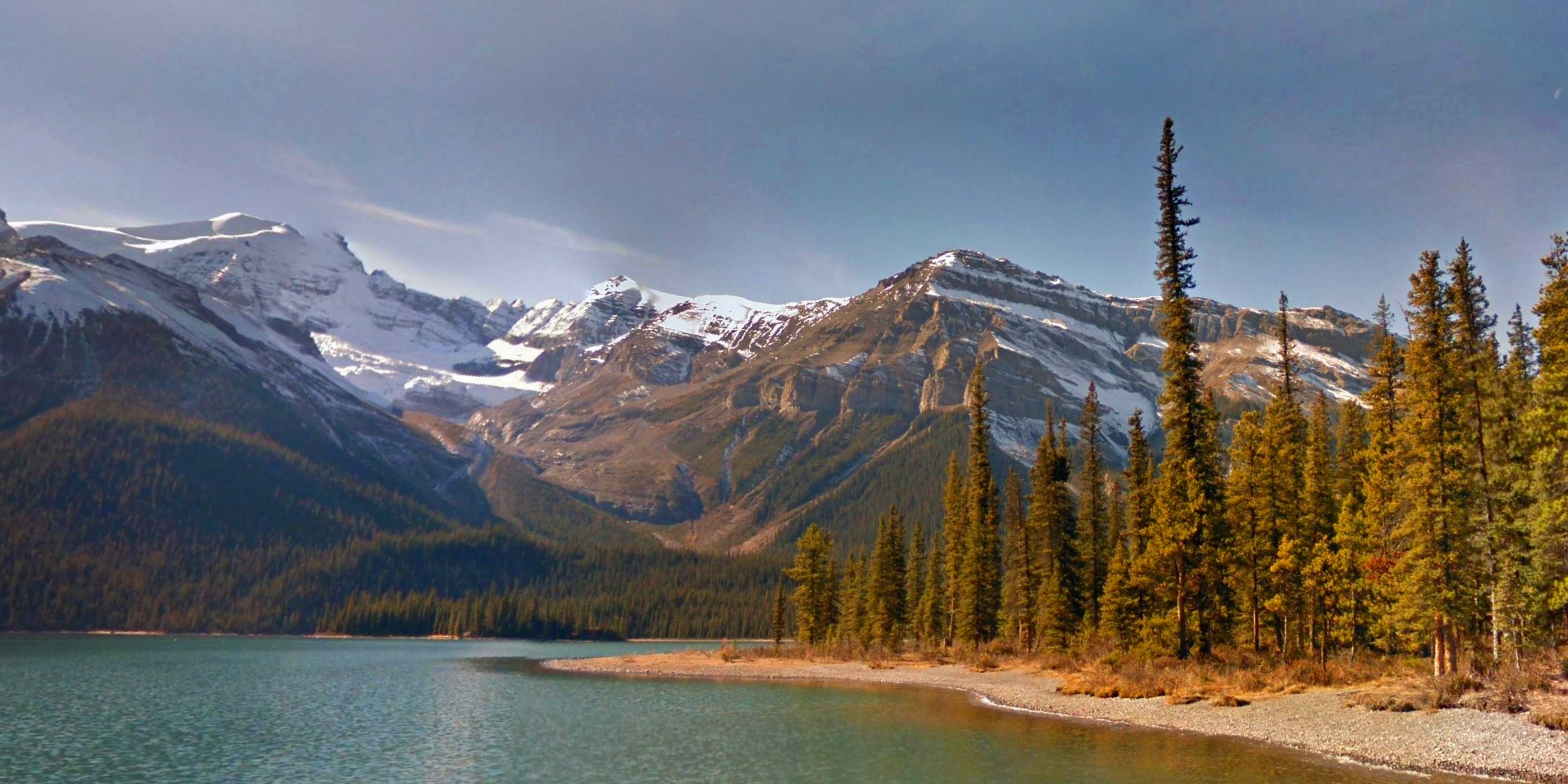
- Source: Twitter
- 798 rows
- 1200 columns
- 3 color channels
- 798 \(\times\) 1,200 \(\times\) 3 \(=\) 2,872,800
- The number of ‘variables’ per image like this!
Using images in practice
- There are a number of strategies to shrink images’ dimensionality
- Downsample the image to a smaller resolution like 256x256x3
- Convert to grayscale
- Cut the image up and use sections of the image as variables instead of individual numbers in the matrix
- Often done with convolutions in neural networks
- Drop variables that aren’t needed, like LASSO
Images in R using Keras
R interface to Keras
By R Studio: details here
- Install with:
devtools::install_github("rstudio/keras") - Finish the install in one of two ways:
For those using Conda
- CPU Based, works on any computer
- Nvidia GPU based
- Install the Software requirements first
Using your own python setup
- Follow Google’s install instructions for Tensorflow
- Install keras from a terminal with
pip install keras - R Studio’s keras package will automatically find it
- May require a reboot to work on Windows
The “hello world” of neural networks
- A “Hello world” is the standard first program one writes in a language
- In R, that could be:
## [1] "Hello world!"- For neural networks, the “Hello world” is writing a handwriting classification script
- We will use the MNIST database, which contains many writing samples and the answers
- Keras provides this for us :)
Set up and pre-processing
- We still do training and testing samples
- It is just as important here as before!
- Shape and scale the data into a big matrix with every value between 0 and 1
Building a Neural Network
model <- keras_model_sequential() # Open an interface to tensorflow
# Set up the neural network
model %>%
    layer_dense(units = 256, activation = 'relu', input_shape = c(784)) %>%
    layer_dropout(rate = 0.4) %>%
    layer_dense(units = 128, activation = 'relu') %>%
    layer_dropout(rate = 0.3) %>%
    layer_dense(units = 10, activation = 'softmax')
That’s it. Keras makes it easy.
- Relu is the same as a call option payoff: \(max(x, 0)\)
- Softmax approximates the \(argmax\) function
- Which input was highest?
The model
- We can just call summary() on the model to see what we built
## Model: "sequential_1"
## ________________________________________________________________________________
## Layer (type)                        Output Shape                    Param #
## ================================================================================
## dense (Dense)                       (None, 256)                     200960
## ________________________________________________________________________________
## dropout (Dropout)                   (None, 256)                     0
## ________________________________________________________________________________
## dense_1 (Dense)                     (None, 128)                     32896
## ________________________________________________________________________________
## dropout_1 (Dropout)                 (None, 128)                     0
## ________________________________________________________________________________
## dense_2 (Dense)                     (None, 10)                      1290
## ================================================================================
## Total params: 235,146
## Trainable params: 235,146
## Non-trainable params: 0
## ________________________________________________________________________________
Compile the model
- Tensorflow doesn’t compute anything until you tell it to
- After we have set up the instructions for the model, we compile it to build our actual model
Running the model
- It takes about 1 minute to run on an Nvidia GTX 1080
Out of sample testing
## $loss
## [1] 0.1117176
##
## $accuracy
## [1] 0.9812
Saving the model
- Saving:
- Loading an already trained model:
More advanced image techniques
How CNNs work
- CNNs use repeated convolution, usually looking at slightly bigger chunks of data each iteration
- But what is convolution? It is illustrated by the following graphs (from Wikipedia):
CNN
- AlexNet (paper)
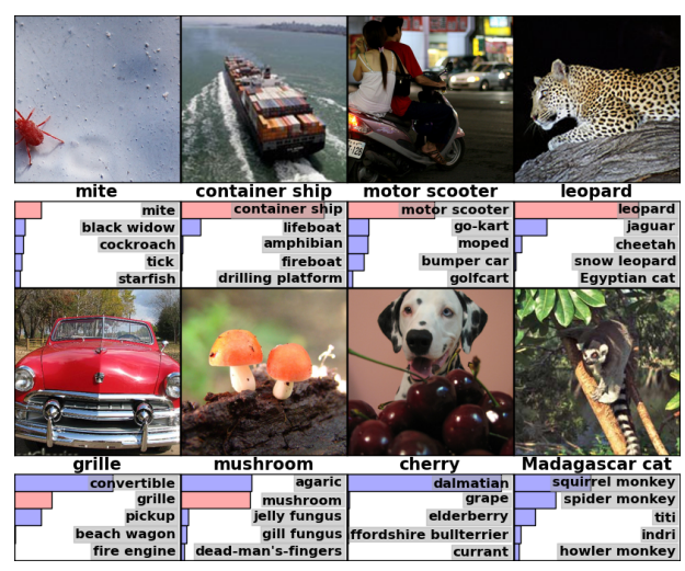
Example output of AlexNet
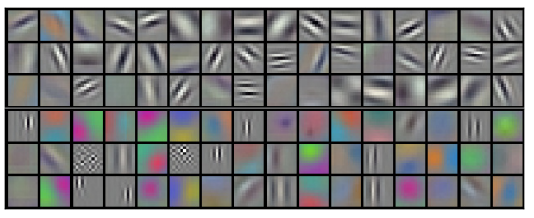
The first (of 5) layers learned
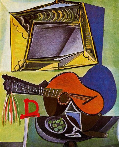
Transfer Learning
- The previous slide is an example of style transfer
- This is also done using CNNs
- More details here
What is transfer learning?
- It is a method of training an algorithm on one domain and then applying the algorithm on another domain
- It is useful when…
- You don’t have enough data for your primary task
- And you have enough for a related task
- You want to augment a model with even more
- You don’t have enough data for your primary task
Try it out!
- Colab file available at this link
- Largely based off of dsgiitr/Neural-Style-Transfer
- It just took a few tweaks to get it working in a Google Colaboratory environment properly
Inputs:
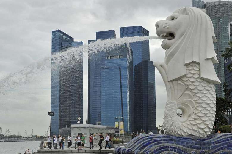
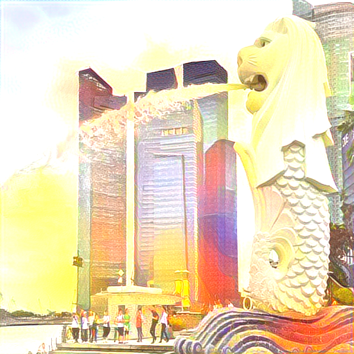
Another generative use: Photography
Input
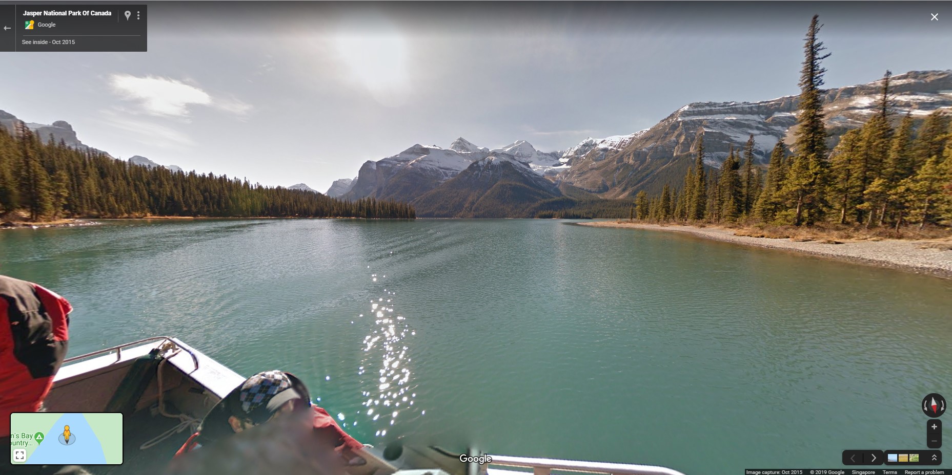
Output
Try out a CNN in your browser!
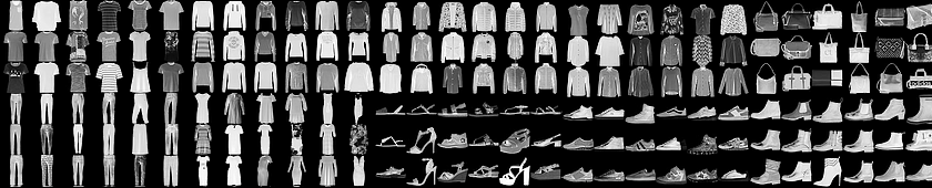
- Fashion MNIST with Keras and TPUs
- Fashion MNIST: A dataset of clothing pictures
- Keras: An easier API for TensorFlow
- TPU: A “Tensor Processing Unit” – A custom processor built by Google
- Python code
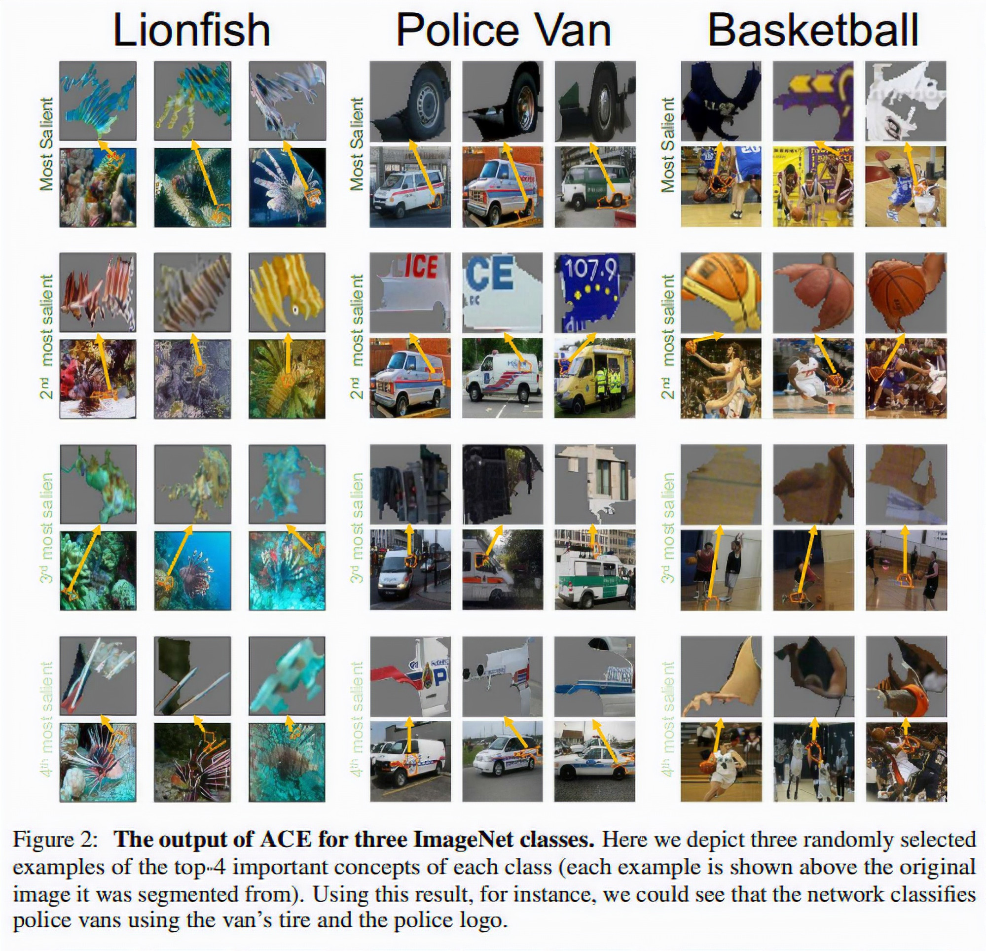
Recent attempts at explaining CNNs
- Google & Stanford’s “Automated Concept-based Explanation”
Detecting financial content
The data
- 5,000 images that should not contain financial information
- 2,777 images that should contain financial information
- 500 of each type are held aside for testing
Goal: Build a classifier based on the images’ content
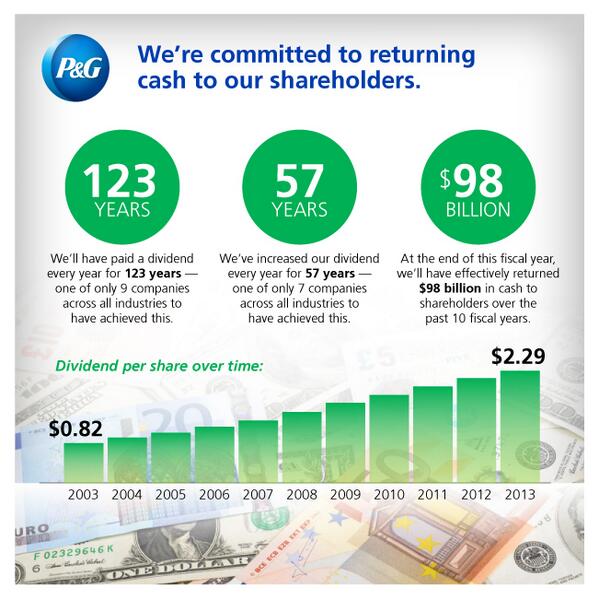
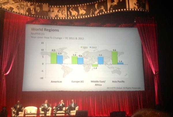
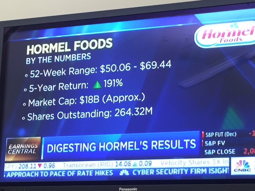
Examples: Financial

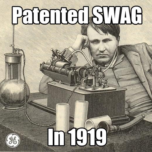
Examples: Non-financial


The CNN
## Model: "sequential"
## ________________________________________________________________________________
## Layer (type)                        Output Shape                    Param #
## ================================================================================
## conv2d (Conv2D)                     (None, 254, 254, 32)            896
## ________________________________________________________________________________
## re_lu (ReLU)                        (None, 254, 254, 32)            0
## ________________________________________________________________________________
## conv2d_1 (Conv2D)                   (None, 252, 252, 16)            4624
## ________________________________________________________________________________
## leaky_re_lu (LeakyReLU)             (None, 252, 252, 16)            0
## ________________________________________________________________________________
## batch_normalization (BatchNormaliza (None, 252, 252, 16)            64
## ________________________________________________________________________________
## max_pooling2d (MaxPooling2D)        (None, 126, 126, 16)            0
## ________________________________________________________________________________
## dropout (Dropout)                   (None, 126, 126, 16)            0
## ________________________________________________________________________________
## flatten (Flatten)                   (None, 254016)                  0
## ________________________________________________________________________________
## dense (Dense)                       (None, 20)                      5080340
## ________________________________________________________________________________
## activation (Activation)             (None, 20)                      0
## ________________________________________________________________________________
## dropout_1 (Dropout)                 (None, 20)                      0
## ________________________________________________________________________________
## dense_1 (Dense)                     (None, 2)                       42
## ________________________________________________________________________________
## activation_1 (Activation)           (None, 2)                       0
## ================================================================================
## Total params: 5,085,966
## Trainable params: 5,085,934
## Non-trainable params: 32
## ________________________________________________________________________________
Running the model
- It takes about 10 minutes to run on an Nvidia GTX 1080
Out of sample testing
eval <- model %>%
  evaluate_generator(img_test,
                     steps = as.integer(test_samples / batch_size),
                     workers = 4)
eval
## $loss
## [1] 0.7535837
##
## $accuracy
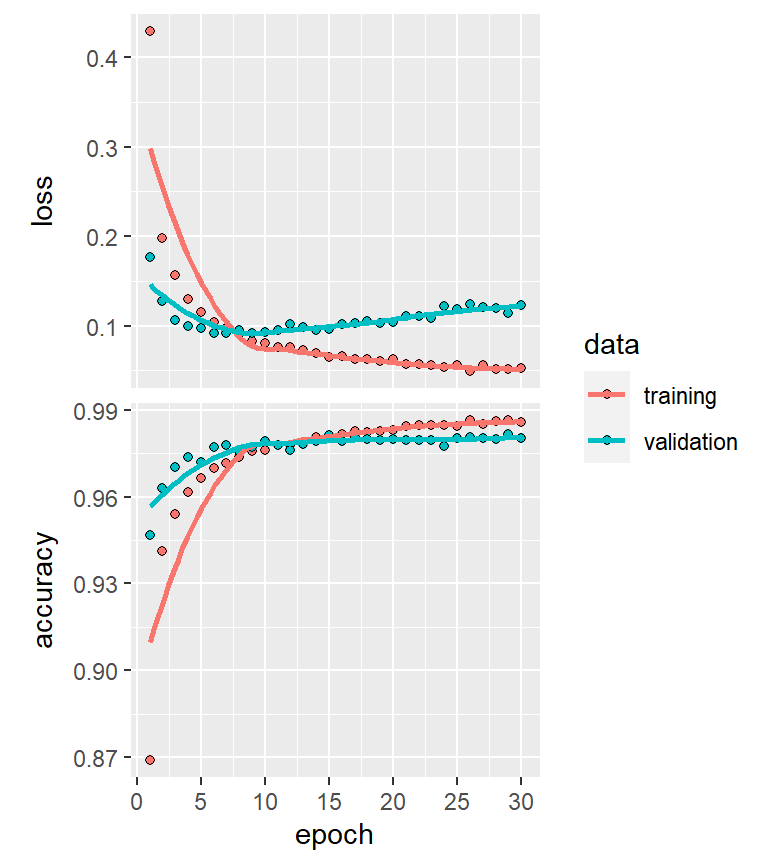
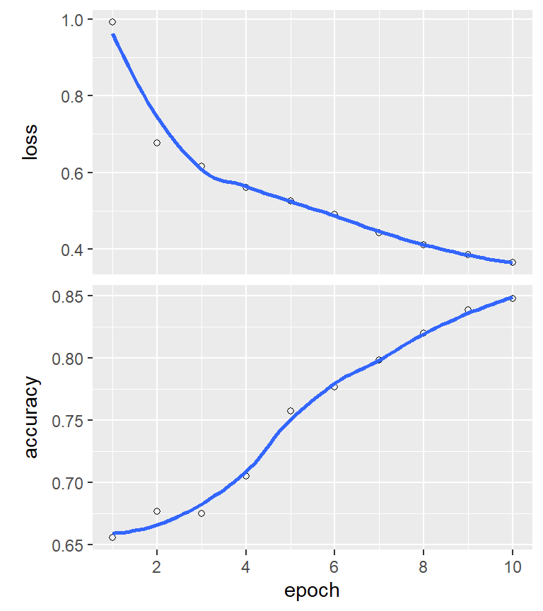
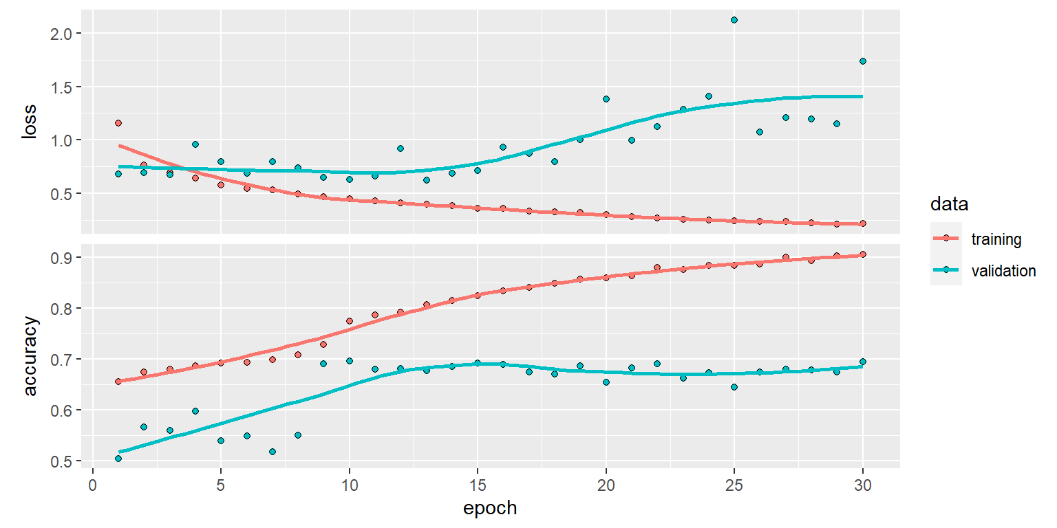
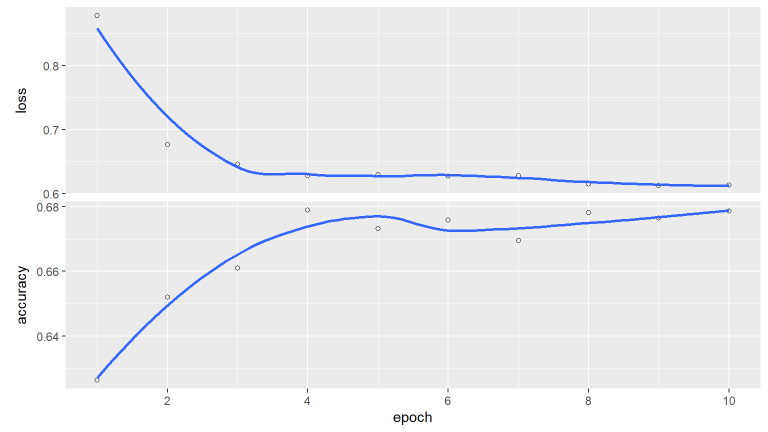
## [1] 0.6572581Optimizing the CNN
- The model we saw was run for 10 epochs (iterations)
- Why not more? Why not less?
AlexNet variant
## Model: "sequential_2"
## ________________________________________________________________________________
## Layer (type)                        Output Shape                    Param #
## ================================================================================
## conv2d_4 (Conv2D)                   (None, 62, 62, 96)              34944
## ________________________________________________________________________________
## re_lu_2 (ReLU)                      (None, 62, 62, 96)              0
## ________________________________________________________________________________
## max_pooling2d_2 (MaxPooling2D)      (None, 31, 31, 96)              0
## ________________________________________________________________________________
## batch_normalization_2 (BatchNormali (None, 31, 31, 96)              384
## ________________________________________________________________________________
## conv2d_5 (Conv2D)                   (None, 21, 21, 256)             2973952
## ________________________________________________________________________________
## re_lu_3 (ReLU)                      (None, 21, 21, 256)             0
## ________________________________________________________________________________
## max_pooling2d_3 (MaxPooling2D)      (None, 10, 10, 256)             0
## ________________________________________________________________________________
## batch_normalization_3 (BatchNormali (None, 10, 10, 256)             1024
## ________________________________________________________________________________
## conv2d_6 (Conv2D)                   (None, 8, 8, 384)               885120
## ________________________________________________________________________________
## re_lu_4 (ReLU)                      (None, 8, 8, 384)               0
## ________________________________________________________________________________
## batch_normalization_4 (BatchNormali (None, 8, 8, 384)               1536
## ________________________________________________________________________________
## conv2d_7 (Conv2D)                   (None, 6, 6, 384)               1327488
## ________________________________________________________________________________
## re_lu_5 (ReLU)                      (None, 6, 6, 384)               0
## ________________________________________________________________________________
## batch_normalization_5 (BatchNormali (None, 6, 6, 384)               1536
## ________________________________________________________________________________
## conv2d_8 (Conv2D)                   (None, 4, 4, 384)               1327488
## ________________________________________________________________________________
## re_lu_6 (ReLU)                      (None, 4, 4, 384)               0
## ________________________________________________________________________________
## max_pooling2d_4 (MaxPooling2D)      (None, 2, 2, 384)               0
## ________________________________________________________________________________
## batch_normalization_6 (BatchNormali (None, 2, 2, 384)               1536
## ________________________________________________________________________________
## flatten_2 (Flatten)                 (None, 1536)                    0
## ________________________________________________________________________________
## dense_4 (Dense)                     (None, 4096)                    6295552
## ________________________________________________________________________________
## activation_4 (Activation)           (None, 4096)                    0
## ________________________________________________________________________________
## dropout_4 (Dropout)                 (None, 4096)                    0
## ________________________________________________________________________________
## batch_normalization_7 (BatchNormali (None, 4096)                    16384
## ________________________________________________________________________________
## dense_5 (Dense)                     (None, 4096)                    16781312
## ________________________________________________________________________________
## activation_5 (Activation)           (None, 4096)                    0
## ________________________________________________________________________________
## dropout_5 (Dropout)                 (None, 4096)                    0
## ________________________________________________________________________________
## batch_normalization_8 (BatchNormali (None, 4096)                    16384
## ________________________________________________________________________________
## dense_6 (Dense)                     (None, 1000)                    4097000
## ________________________________________________________________________________
## activation_6 (Activation)           (None, 1000)                    0
## ________________________________________________________________________________
## dropout_6 (Dropout)                 (None, 1000)                    0
## ________________________________________________________________________________
## batch_normalization_9 (BatchNormali (None, 1000)                    4000
## ________________________________________________________________________________
## dense_7 (Dense)                     (None, 2)                       2002
## ________________________________________________________________________________
## activation_7 (Activation)           (None, 2)                       0
## ================================================================================
## Total params: 33,767,642
## Trainable params: 33,746,250
## Non-trainable params: 21,392
## ________________________________________________________________________________
AlexNet performance
Video data
Working with video
- Video data is challenging – very storage intensive
- Ex.: Uber’s self driving cars would generate >100GB of data per hour per car
- Video data is very promising
- Think of how many task involve vision!
- Driving
- Photography
- Warehouse auditing…
- Think of how many task involve vision!
- At the end of the day though, video is just a sequence of images
One method for video
YOLOv3
- You
- Only
- Once
What does YOLO do?
- It spots objects in videos and labels them
- It also figures out a bounding box – a box containing the object inside the video frame
- It can spot overlapping objects
- It can spot multiple of the same or different object types
- The baseline model (using the COCO dataset) can detect 80 different object types
- There are other datasets with more objects
How does Yolo do it? Map of Tiny YOLO
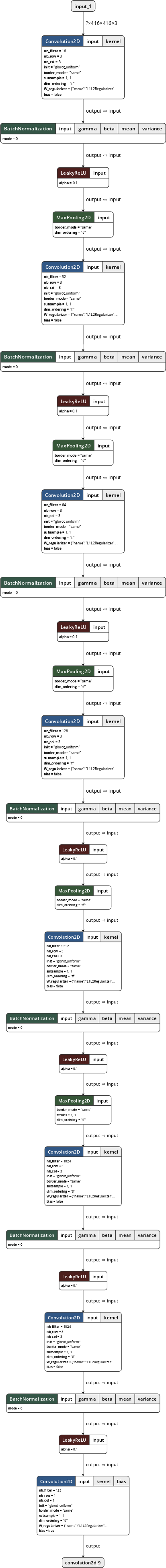
Yolo model and graphing tool from lutzroeder/netron
How does Yolo do it?
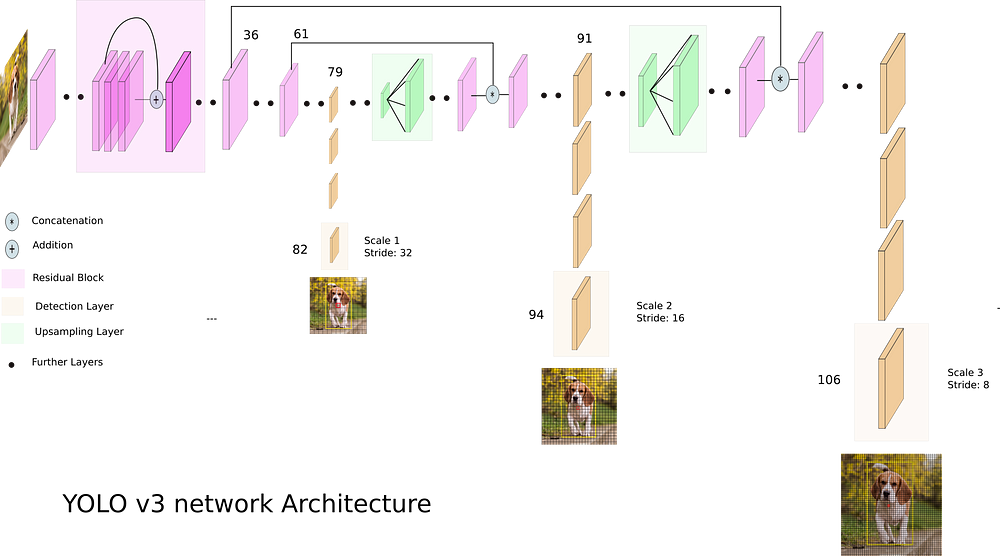
Diagram from What’s new in YOLO v3 by Ayoosh Kathuria
Final word on object detection
- An algorithm like YOLO v3 is somewhat tricky to run
- Preparing the algorithm takes a long time
- The final output, though, can run on much cheaper hardware
- These algorithms just recently became feasible so their impact has yet to be felt so strongly
Think about how facial recognition showed up everywhere for images over the past few years
Where to get video data
- One extensive source is Youtube-8M
- 6.1M videos, 3-10 minutes each
- Each video has >1,000 views
- 350,000 hours of video
- 237,000 labeled 5 second segments
- 1.3B video features that are machine labeled
- 1.3B audio features that are machine labeled
End matter
Final discussion
What creative uses for the techniques discussed today do you expect to see become reality in accounting in the next 3-5 years?
- 1 example: Using image recognition techniques, warehouse counting for audit can be automated
- Strap a camera to a drone, have it fly all over the warehouse, and process the video to get item counts
Recap
Today, we:
- Learned about using images as data
- Constructed a simple handwriting recognition system
- Learned about more advanced image methods
- Applied CNNs to detect financial information in images on Twitter
- Learned about object detection in videos
For next week
- For next week:
- Finish the group project!
- Kaggle submission closes Sunday!
- Turn in your code, presentation, and report through eLearn’s dropbox
- Prepare a short (~15 minute) presentation for class
- Finish the group project!
More fun examples
- Interactive:
- Others:
Fun machine learning examples
- Interactive:
- Draw together with a neural network
- click the images to try it out yourself!
- Google’s Quickdraw
- Google’s Teachable Machine
- Four experiments in handwriting with a neural network
- Draw together with a neural network
Bonus: Neural networks in interactive media
- Super Mario using MarI/O
- Mario Kart using an RNN for controller prediction
- Open AI’s Five tops Dota 2
- Trained on 180 years of play
- Google Deepmind’s Alphastar AI on StarCraft II
- Trained on 200 years of play