Learning objectives
- Theory:
- Develop a logical approach to problem solving with data
- Statistics
- Causation
- Hypothesis testing
- Develop a logical approach to problem solving with data
- Application:
- Predicting revenue for real estate firms
- Methodology:
- Univariate stats
- Linear regression
- Visualization
R Markdown: A quick guide
- Headers and subheaders start with
#and##, respectively - Code blocks starts with
```{r}and end with```- By default, all code and figures will show up in the document
- Inline code goes in a block starting with
`rand ending with` - Italic font can be used by putting
*or_around text - Bold font can be used by putting
**around text- E.g.:
**bold text**becomes bold text
- E.g.:
- To render the document, click

- Math can be placed between
$to use LaTeX notation- E.g.
$\frac{revt}{at}$becomes \(\frac{revt}{at}\)
- E.g.
- Full equations (on their own line) can be placed between
$$ - A block quote is prefixed with
> - For a complete guide, see R Studio’s R Markdown::Cheat Sheet
The question
How can we predict revenue for a company, leveraging data about that company, related companies, and macro factors
- Specific application: Real estate companies

Example
Let’s predict UOL’s revenue for 2016


- Compustat has data for them since 1989
- Complete since 1994
- Missing CapEx before that
- Complete since 1994
##       revt               at
##  Min.   :  94.78   Min.   : 1218
##  1st Qu.: 193.41   1st Qu.: 3044
##  Median : 427.44   Median : 3478
##  Mean   : 666.38   Mean   : 5534
##  3rd Qu.:1058.61   3rd Qu.: 7939
## Max. :2103.15 Max. :19623Why is it called Ordinary Least Squares?
Frequentist vs Bayesian methods
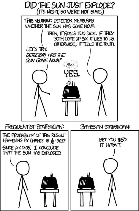
This is why we use more than 1 data point
Mental model of OLS: 1 input
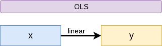
Simple OLS measures a simple linear relationship between an input and an output
- E.g.: Our first regression this week: Revenue on assets
Mental model of OLS: Multiple inputs
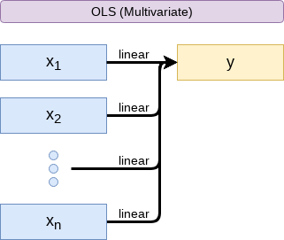
OLS measures simple linear relationships between a set of inputs and one output
- E.g.: This is what we did when scaling up earlier this session
Other linear models: IV Regression (2SLS)
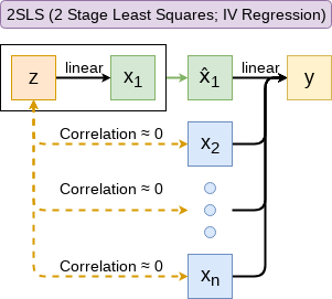
IV/2SLS models linear relationships where the effect of some \(x_i\) on \(y\) may be confounded by outside factors.
- E.g.: Modeling the effect of management pay duration (like bond duration) on firms’ choice to issue earnings forecasts
- Instrument with CEO tenure (Cheng, Cho, and Kim 2015)
Other linear models: SUR
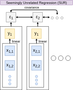
SUR models systems with related error terms
- E.g.: Modeling both revenue and earnings simultaneously
Other linear models: 3SLS
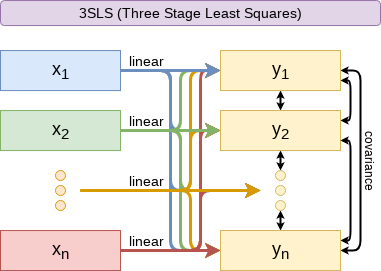
3SLS models systems of equations with related outputs
- E.g.: Modeling stock return, volatility, and volume simultaneously
Other linear models: SEM
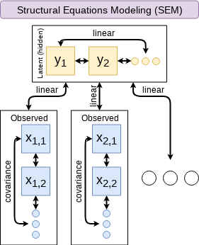
SEM can model abstract and multi-level relationships
- E.g.: Showing that organizational commitment leads to higher job satisfaction, not the other way around (Poznanski and Bline 1999)
Modeling choices: Variable selection
- The options:
- Use your own knowledge to select variables
- Use a selection model to automate it
Own knowledge
- Build a model based on your knowledge of the problem and situation
- This is generally better
- The result should be more interpretable
- For prediction, you should know relationships better than most algorithms

Modeling choices: Automated selection
- Traditional methods include:
- Forward selection: Start with nothing and add variables with the most contribution to Adj \(R^2\) until it stops going up
- Backward selection: Start with all inputs and remove variables with the worst (negative) contribution to Adj \(R^2\) until it stops going up
- Stepwise selection: Like forward selection, but drops non-significant predictors
- Newer methods:
- Lasso and Elastic Net based models
- Optimize with high penalties for complexity (i.e., # of inputs)
- We will discuss these in week 5
- Lasso and Elastic Net based models

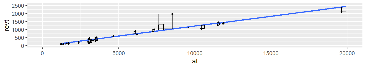
Coefficients
- In OLS: \(\beta_i\)
- A change in \(x_i\) by 1 leads to a change in \(y\) by \(\beta_i\)
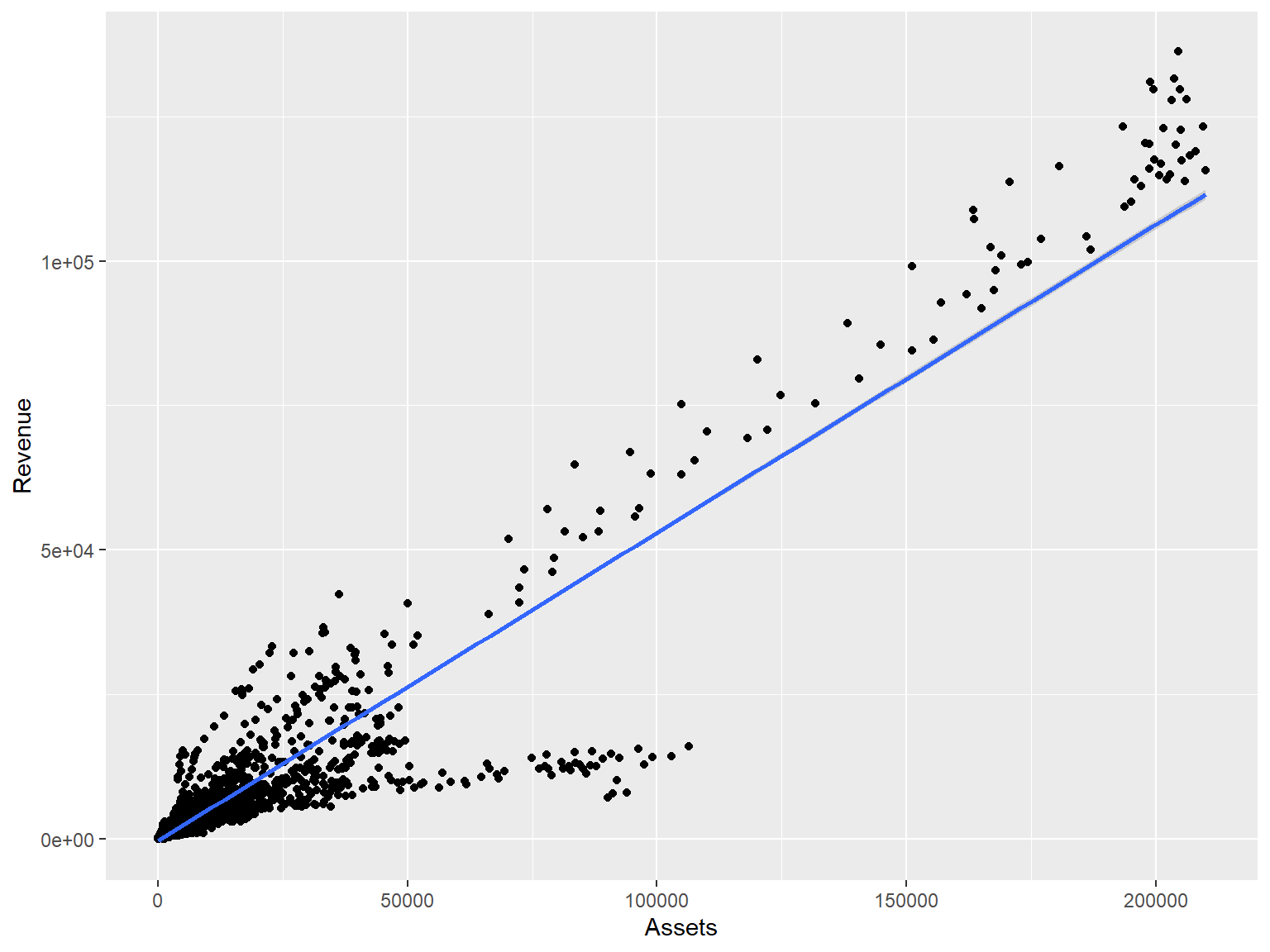
- Essentially, the slope between \(x\) and \(y\)
- The blue line in the chart is the regression line for \(\hat{Revenue} = \alpha + \beta_i \hat{Assets}\) for retail firms since 1960
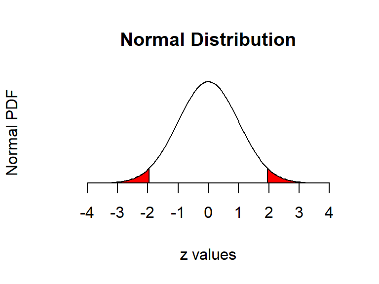
One vs two tailed tests
- Best practice:
- Use a two tailed test
- Second best practice:
- If you use a 1-tailed test, use a p-value cutoff of 0.025 or 0.05
- This is equivalent to the best practice, just roundabout
- If you use a 1-tailed test, use a p-value cutoff of 0.025 or 0.05
- Common but generally inappropriate:
- Use a one tailed test with cutoffs of 0.05 or 0.10 because your hypothesis is directional
What is causality?
\(A \rightarrow B\)
- Causality is \(A\) causing \(B\)
- This means more than \(A\) and \(B\) are correlated
- I.e., If \(A\) changes, \(B\) changes. But \(B\) changing doesn’t mean \(A\) changed
- Unless \(B\) is 100% driven by \(A\)
- Very difficult to determine, particularly for events that happen [almost] simultaneously
- Examples of correlations that aren’t causation

Time and causality break down
\(A_t \rightarrow B_{t+1}\)? \(\quad\) OR \(\quad\) \(C \rightarrow A_t\) and \(C \rightarrow B_{t+1}\)?
- The above illustrates the Correlated omitted variable problem
- \(A\) doesn’t cause \(B\)… Instead, some other force \(C\) causes both
- The bane of social scientists everywhere
- This is less important for predictive analytics, as we care more about performance, but…
- It can complicate interpreting your results
- Figuring out \(C\) can help improve you model’s predictions
- So find C!

Panel data
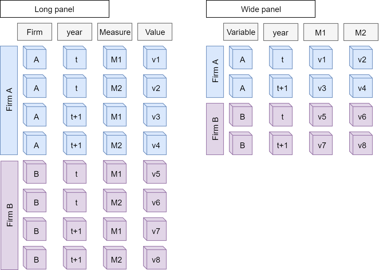
Data frames are usually wide panels
All Singapore real estate companies
# Note the group_by -- without it, lead() will pull from the subsequent firm!
# ungroup() tells R that we finished grouping
df_clean <- df_clean %>%
  group_by(isin) %>%
  mutate(revt_lead = lead(revt)) %>%
  ungroup()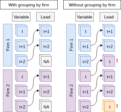
Why exactly would we use fixed effects?
- Fixed effects are used when the average of \(\hat{y}\) varies by some group in our data
- In our problem, the average revenue of each firm is different
- Fixed effects absorb this difference
- Further reading:
- Introductory Econometrics by Jeffrey M. Wooldridge