ACCT 420: R Supplement
Session 1 Supplement
Dr. Richard M. Crowley
rcrowley@smu.edu.sg
http://rmc.link/
Vectors
Vectors: What are they?
- Remember back to linear algebra…
Examples:
\[ \begin{matrix} \left(\begin{matrix} 1 \\ 2 \\ 3 \\ 4 \end{matrix}\right) & \text{or} & \left(\begin{matrix} 1 & 2 & 3 & 4 \end{matrix}\right) \end{matrix} \]
A row (or column) of data
Vector creation
- Vectors are entered using the c() command
- Any data type is fine, but all elements must be the same type
## [1] "Google" "Microsoft" "Goldman"## [1] TRUE TRUE FALSE## [1] 12662 21204 4286A vector in R is a 1 dimensional collection of 1 or more of the same data type
Special cases for vectors
- Counting between integers
:, e.g.1:5or22:500- seq(), e.g.
seq(from=0, to=100,by=5)
## [1] 1 2 3 4 5## [1] 0 5 10 15 20 25 30 35 40 45 50 55 60 65 70 75 80 85 90
## [20] 95 100\(\uparrow\) note that [18] means the 18th output
- Repeating something
- rep(), e.g.
rep(1,times=10)orrep("hi",times=5)
- rep(), e.g.
## [1] 1 1 1 1 1 1 1 1 1 1## [1] "hi" "hi" "hi" "hi" "hi"Vector math
Works the same as scalars, but applies element-wise
- First element with first element,
- Second element with second element,
- …
## [1] 12662 21204 4286## [1] 25324 42408 8572## [1] 160326244 449609616 18369796Vector math
Can also use 1 vector and 1 scalar
- Scalar is applied to all vector elements
## [1] 22662 31204 14286## [1] 22662 31204 14286## [1] 12.662 21.204 4.286Vector math
- From linear algebra remember multiplication as a dot product. That can be done with
%*%
##           [,1]
## [1,] 628305656## [1] 628305656## [1] 3## [1] 38152Naming vectors
- Vectors allow us to include a lot of information in one object
- It isn’t easy to read though
- We can make things more readable by assigning names()
- Names provide a way to easily work with and understand the data
Selecting and combining vectors
- Selecting can be done a few ways.
- By index, such as
[1] - By name, such as
["Google"]
- By index, such as
## Google
## 12662## Google
## 12662- Multiple selection:
earnings[c(1,2)]earnings[1:2]earnings[c("Google","Microsoft")]
##    Google Microsoft
## 12662 21204- Combining is done using c()
## [1] 1 2 3 4 5 6Vector example: Profit margin for tech firms
# Calculating proit margin for all public US tech firms
# 715 tech firms with >1M sales in 2017
summary(earnings_2017)  # Cleaned data from Compustat, in $M USD
## Min. 1st Qu. Median Mean 3rd Qu. Max.
## -4307.49 -15.98 1.84 296.84 91.36 48351.00## Min. 1st Qu. Median Mean 3rd Qu. Max.
## 1.06 102.62 397.57 3023.78 1531.59 229234.00## Min. 1st Qu. Median Mean 3rd Qu. Max.
## -13.97960 -0.10253 0.01353 -0.10967 0.09295 1.02655Practice: Vectors
- This practice explores the ROA of Goldman Sachs, JPMorgan, and Citigroup in 2017
- Do exercise 2 on the supplementary R practice file:
Matrices
Matrices: What are they?
- Remember back to linear algebra…
Example:
\[ \left(\begin{matrix} 1 & 2 & 3 & 4\\ 5 & 6 & 7 & 8\\ 9 & 10 & 11 & 12 \end{matrix}\right) \]
A rows and columns of data
Matrix creation
- Matrices are entered using the matrix() command
- Any data type is fine, but all elements must be the same type
columns <- c("Google", "Microsoft", "Goldman")
rows <- c("Earnings","Revenue")

# equivalent: matrix(data=c(12662, 21204, 4286, 110855, 89950, 42254),ncol=3)
firm_data <- matrix(data=c(12662, 21204, 4286, 110855, 89950, 42254),nrow=2)
firm_data
## [,1] [,2] [,3]
## [1,] 12662 4286 89950
## [2,] 21204 110855 42254Math with matrices
Everything with matrices works just like vectors
##       [,1]   [,2]   [,3]
## [1,] 25324   8572 179900
## [2,] 42408 221710 84508## [,1] [,2] [,3]
## [1,] 12.662 4.286 89.950
## [2,] 21.204 110.855 42.254Matrix math with matrices
- Matrix transposing, \(A^T\), uses t()
##       [,1]   [,2]
## [1,] 12662  21204
## [2,]  4286 110855
## [3,] 89950 42254- Matrix multiplication, \(A~B\), uses
%*%
##            [,1]        [,2]
## [1,] 8269698540  4544356878
## [2,] 4544356878 14523841157
We won’t use these much, but they can be useful
Matrix naming
- We can name matrix rows and columns, much like we named vector elements
- Use rownames() for rows
- Use colnames() for columns
##          Google Microsoft Goldman
## Earnings  12662      4286   89950
## Revenue   21204    110855   42254
Selecting from matrices
- Select using 2 indexes instead of 1:
matrix_name[rows,columns]- To select all rows or columns, leave that index blanks
## [1] 42254## Google Microsoft
## Earnings 12662 4286
## Revenue 21204 110855## Google Microsoft Goldman
## 12662 4286 89950Combining matrices
- Matrices are combined top to bottom as rows with rbind()
- Matrices are combined side-by-side as columns with cbind()
# Preloaded: industry codes as indcode (vector)
#     - GICS codes: 40=Financials, 45=Information Technology
#     - See: https://en.wikipedia.org/wiki/Global_Industry_Classification_Standard
# Preloaded: JPMorgan data as jpdata (vector)

mat <- rbind(firm_data,indcode)  # Add a row
rownames(mat)[3] <- "Industry"  # Name the new row
mat
## Google Microsoft Goldman
## Earnings 12662 4286 89950
## Revenue 21204 110855 42254
## Industry 45 45 40mat <- cbind(firm_data,jpdata) # Add a column
colnames(mat)[4] <- "JPMorgan" # Name the new column
mat## Google Microsoft Goldman JPMorgan
## Earnings 12662 4286 89950 17370
## Revenue 21204 110855 42254 115475Lists
Lists: What are they?
- Like vectors, but with mixed types
- Generally not something we will create
- Often returned by analysis functions in R
- Such as the linear models we will look at next week
# Ignore this code for now...
model <- summary(lm(earnings ~ revenue, data=tech_df))
#Note that this function is hiding something...
model
##
## Call:
## lm(formula = earnings ~ revenue, data = tech_df)
##
## Residuals:
## Min 1Q Median 3Q Max
## -16045.0 20.0 141.6 177.1 12104.6
##
## Coefficients:
## Estimate Std. Error t value Pr(>|t|)
## (Intercept) -1.837e+02 4.491e+01 -4.091 4.79e-05 ***
## revenue 1.589e-01 3.564e-03 44.585 < 2e-16 ***
## ---
## Signif. codes: 0 '***' 0.001 '**' 0.01 '*' 0.05 '.' 0.1 ' ' 1
##
## Residual standard error: 1166 on 713 degrees of freedom
## Multiple R-squared: 0.736, Adjusted R-squared: 0.7356
## F-statistic: 1988 on 1 and 713 DF, p-value: < 2.2e-16Looking into lists
- Lists generally use double square brackets,
[[index]]- Used for pulling individual elements out of a list
[[c()]]will drill through lists, as opposed to pulling multiple values- Single square brackets pull out elements as is
- Double square brackets extract just the element
- For 1 level, we can also use
$
Structure of a list
- str() will tell us what’s in this list
## List of 11
##  $ call         : language lm(formula = earnings ~ revenue, data = tech_df)
##  $ terms        :Classes 'terms', 'formula'  language earnings ~ revenue
##   .. ..- attr(*, "variables")= language list(earnings, revenue)
##   .. ..- attr(*, "factors")= int [1:2, 1] 0 1
##   .. .. ..- attr(*, "dimnames")=List of 2
##   .. .. .. ..$ : chr [1:2] "earnings" "revenue"
##   .. .. .. ..$ : chr "revenue"
##   .. ..- attr(*, "term.labels")= chr "revenue"
##   .. ..- attr(*, "order")= int 1
##   .. ..- attr(*, "intercept")= int 1
##   .. ..- attr(*, "response")= int 1
##   .. ..- attr(*, ".Environment")=<environment: R_GlobalEnv>
##   .. ..- attr(*, "predvars")= language list(earnings, revenue)
##   .. ..- attr(*, "dataClasses")= Named chr [1:2] "numeric" "numeric"
##   .. .. ..- attr(*, "names")= chr [1:2] "earnings" "revenue"
##  $ residuals    : Named num [1:715] -59.7 173.8 -620.2 586.7 613.6 ...
##   ..- attr(*, "names")= chr [1:715] "1" "2" "3" "4" ...
##  $ coefficients : num [1:2, 1:4] -1.84e+02 1.59e-01 4.49e+01 3.56e-03 -4.09 ...
##   ..- attr(*, "dimnames")=List of 2
##   .. ..$ : chr [1:2] "(Intercept)" "revenue"
##   .. ..$ : chr [1:4] "Estimate" "Std. Error" "t value" "Pr(>|t|)"
##  $ aliased      : Named logi [1:2] FALSE FALSE
##   ..- attr(*, "names")= chr [1:2] "(Intercept)" "revenue"
##  $ sigma        : num 1166
##  $ df           : int [1:3] 2 713 2
##  $ r.squared    : num 0.736
##  $ adj.r.squared: num 0.736
##  $ fstatistic   : Named num [1:3] 1988 1 713
##   ..- attr(*, "names")= chr [1:3] "value" "numdf" "dendf"
##  $ cov.unscaled : num [1:2, 1:2] 1.48e-03 -2.83e-08 -2.83e-08 9.35e-12
##   ..- attr(*, "dimnames")=List of 2
##   .. ..$ : chr [1:2] "(Intercept)" "revenue"
##   .. ..$ : chr [1:2] "(Intercept)" "revenue"
##  - attr(*, "class")= chr "summary.lm"
Practice: Lists
- In this practice, we will explore lists and how to parse them
- Do exercise 3 on the supplementary R practice file:
Data frames
What are data frames?
- Data frames are like a hybrid between lists and matrices
Like a matrix:
- 2 dimensional like matrices
- Can access data with
[] - All elements in a column must be the same data type
Like a list:
- Can have different data types for different columns
- Can access data with
$
Think of columns as variables, rows as observations
Example of a data frame
How to create data frames
- On import of data, usually you will get a data frame
- Using the data.frame() function
##           companyName earnings tech_firm
## Google         Google    12662      TRUE
## Microsoft   Microsoft    21204      TRUE
## Goldman       Goldman     4286     FALSE
Note:
stringsAsFactors=FALSEis no longer needed as of R 4.0.0
Selecting from data frames
- Access like a matrix
## [1] "Google" "Microsoft" "Goldman"- Access like a list
## [1] "Google" "Microsoft" "Goldman"## [1] "Google" "Microsoft" "Goldman"All are relatively equivalent. Using
$is generally most natural. Using[,]is good for complex references.
Making new columns in a data frame
Suggested method: use
$
df$all_zero <- 0
df$revenue <- c(110855, 89950, 42254)
df$margin <- df$earnings / df$revenue
# Custom function for small tables -- see last slide for code
html_df(df)| companyName | earnings | tech_firm | all_zero | revenue | margin | |
|---|---|---|---|---|---|---|
| 12662 | TRUE | 0 | 110855 | 0.1142213 | ||
| Microsoft | Microsoft | 21204 | TRUE | 0 | 89950 | 0.2357310 |
| Goldman | Goldman | 4286 | FALSE | 0 | 42254 | 0.1014342 |
Alternative method: use cbind() just like with matrices
Sorting data frames
- To sort a vector, we could use the sort()
## [1] 4286 12662 21204THIS CAN’T SORT DATA FRAMES
- A column of a data frame is fine, but it can’t sort the whole thing!
Sorting data frames
- To sort a data frame, we use the order() function
- It returns the order of each element in increasing value
- 1 is the lowest value
- Then we pass the new order like we are selecting elements
- It returns the order of each element in increasing value
## [1] 3 1 2## companyName earnings tech_firm all_zero revenue margin
## Goldman Goldman 4286 FALSE 0 42254 0.1014342
## Google Google 12662 TRUE 0 110855 0.1142213
## Microsoft Microsoft 21204 TRUE 0 89950 0.2357310Sorting data frames
- Order can sort by multiple levels
order(level1,level2,...), wherelevel_are vectors or data frame columns
# Example of multicolumn sorting:
example <- data.frame(firm=c("Google","Microsoft","Google","Microsoft"),
                      year=c(2017,2017,2016,2016))
example
## firm year
## 1 Google 2017
## 2 Microsoft 2017
## 3 Google 2016
## 4 Microsoft 2016# with() allows us to avoiding prepending each column with "example$"
ordering <- order(example$firm, example$year)
example <- example[ordering,]
example## firm year
## 3 Google 2016
## 1 Google 2017
## 4 Microsoft 2016
## 2 Microsoft 2017Subsetting data frames
- We can use the selecting methods from before
- We can pass a vector of logical values telling R what to keep
- This is pretty useful!
##           companyName earnings tech_firm all_zero revenue    margin
## Google         Google    12662      TRUE        0  110855 0.1142213
## Microsoft Microsoft 21204 TRUE 0 89950 0.2357310- We can use the subset() function
- I don’t recommend this function, as it does not always work
- There are times where it is useful though
- I don’t recommend this function, as it does not always work
##         companyName earnings tech_firm all_zero revenue    margin
## Goldman     Goldman     4286     FALSE        0   42254 0.1014342
## Google       Google    12662      TRUE        0  110855 0.1142213
Practice: Data frames
- This exercise explores the nature of banks’ deposits
- We will see which of Goldman, JPMorgan, and Citigroup have (since 2010):
- The least of their assets in deposits
- The most of their assets in deposits
- We will see which of Goldman, JPMorgan, and Citigroup have (since 2010):
- Do exercise 4 on the supplementary R practice file:
Logical expressions
Why use logical expressions?
- We just saw an example in our subsetting function
earnings < 20000
- Logical expressions give us more control over the data
- They let us easily create logical vectors for subsetting data
## [1] 4286 12662 21204## [1] TRUE TRUE FALSELogical operators
== != > < >= <= ! | &
- Equals:
==2 == 2\(\rightarrow\) TRUE2 == 3\(\rightarrow\) FALSE'dog'=='dog'\(\rightarrow\) TRUE'dog'=='cat'\(\rightarrow\) FALSE
- Not equals:
!=- The opposite of
== 2 != 2\(\rightarrow\) FALSE2 != 3\(\rightarrow\) TRUE'dog'!='cat'\(\rightarrow\) TRUE
- The opposite of
- Comparing strings is done character by character
- Be very careful with it
Logical operators
== != > < >= <= ! | &
- Greater than:
>2 > 1\(\rightarrow\) TRUE2 > 2\(\rightarrow\) FALSE2 > 3\(\rightarrow\) FALSE'dog'>'cat'\(\rightarrow\) TRUE
- Less than:
>2 < 1\(\rightarrow\) FALSE2 < 2\(\rightarrow\) FALSE2 < 3\(\rightarrow\) TRUE'dog'<'cat'\(\rightarrow\) FALSE
- Greater than or equal to:
>2 >= 1\(\rightarrow\) TRUE2 >= 2\(\rightarrow\) TRUE2 >= 3\(\rightarrow\) FALSE
- Less than or equal to:
>2 <= 1\(\rightarrow\) FALSE2 <= 2\(\rightarrow\) TRUE2 <= 3\(\rightarrow\) TRUE
Logical operators
- Not:
!- This simply inverts everything
!TRUE\(\rightarrow\) FALSE!FALSE\(\rightarrow\) TRUE
- And:
&TRUE & TRUE\(\rightarrow\) TRUETRUE & FALSE\(\rightarrow\) FALSEFALSE & FALSE\(\rightarrow\) FALSE
- Or:
|(pipe, same key as ‘\’)- Note that
|is evaluated after all&s TRUE | TRUE\(\rightarrow\) TRUETRUE | FALSE\(\rightarrow\) TRUEFALSE | FALSE\(\rightarrow\) FALSE
- Note that
- You can mix in parentheses for grouping as needed
Examples for logical operators
- How many tech firms had >$10B in revenue in 2017?
## [1] 46- How many tech firms had >$10B in revenue but had negative earnings in 2017?
## [1] 4- Who are those 4 with high revenue and negative earnings?
columns <- c("conm","tic","earnings","revenue")
tech_df[tech_df$revenue > 10000 & tech_df$earnings < 0, columns]
## conm tic earnings revenue
## 35 CORNING INC GLW -497.000 10116.00
## 45 TELEFONAKTIEBOLAGET LM ERICS ERIC -4307.493 24629.64
## 120 DELL TECHNOLOGIES INC 7732B -3728.000 78660.00
## 214 NOKIA CORP NOK -1796.087 27917.49Other special values
- We know
TRUEandFALSEalready- Note that
FALSEcan be represented as 0 - Note that
TRUEcan be represented as any non-zero number
- Note that
- There are also:
Inf: Infinity, often caused by dividing something by 0NaN: “Not a number,” likely that the expression 0/0 occurredNA: A missing value, usually not due to a mathematical errorNull: Indicates a variable has nothing in it
- We can check for these with:
Practice: Subsetting our data frame
- This practice focuses on subsetting out potentially interesting parts of our data frame
- We will also see which of Goldman, JPMorgan, and Citigroup, in which year, had the lowest earnings since 2010
- Do exercise 5 on the supplementary R practice file:
Other uses
- Conditional statements (used for programming)
# cond1, cond2, etc. can be any logical expression
if(cond1) {
  # Code runs if cond1 is TRUE
} else if (cond2) { # Can repeat 'else if' as needed
  # Code runs if this is the first condition that is TRUE
} else {
  # Code runs if none of the above conditions TRUE
}- Vectorized conditional statements using ifelse()
- If else takes 3 vectors and returns 1 vector
- A vector of
TRUEorFALSE - A vector of elements to return from when
TRUE - A vector of elements to return from when
FALSE
- A vector of
- If else takes 3 vectors and returns 1 vector
# Outputs odd for odd numbers and even for even numbers
even <- rep("even",5)
odd <- rep("odd",5)
numbers <- 1:5
ifelse(numbers %% 2, odd, even)
## [1] "odd" "even" "odd" "even" "odd"Loops and apply
Looping: While loop
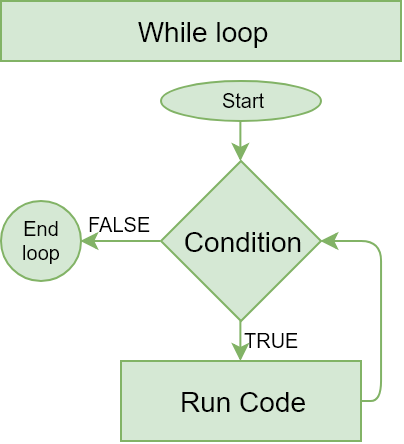
- A while() loop executes code repeatedly until a specified condition is
FALSE
## [1] 0
## [1] 2
## [1] 4
Looping: For loop
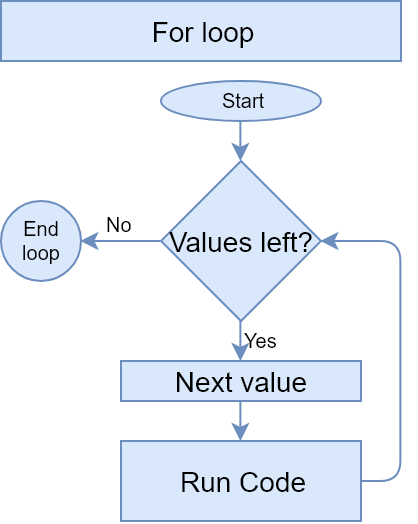
- A for() loop executes code repeatedly until a specified condition is
FALSE, while incrementing a given variable
## [1] 0
## [1] 2
## [1] 4
Dangers of looping in R
- Loops in R are very slow – they do one calculation at a time, but R is best for doing many calculations at once
## [1] TRUE## [1] "4.50333810205055 times"Useful functions
Help functions
- There are two equivalent ways to quickly access help files:
?and help()- Usage to get the help file for data.frame():
?data.framehelp(data.frame)
- To see the options for a function, use args()
## function (..., row.names = NULL, check.rows = FALSE, check.names = TRUE,
##     fix.empty.names = TRUE, stringsAsFactors = FALSE)
## NULL
A note on using functions
## function (..., row.names = NULL, check.rows = FALSE, check.names = TRUE,
##     fix.empty.names = TRUE, stringsAsFactors = FALSE)
## NULL- The
...represents a series of inputs- In this case, inputs like
name=data, where name is the column name and data is a vector
- In this case, inputs like
- The
____ = ____arguments are options for the function- The default is prespecified, but you can overwrite it
- Options can be very useful or save us a lot of time!
- You can always find them by:
- Using the
?command - Checking other documentation like www.rdocumentation.org
- Using the args() function
- Using the
Installing more functions
- R Provides an easy way to install packages without ever leaving R
- The install.packages() command
- Can install a single package or a vector of packages
# To install the tidyverse package:
install.packages("tidyverse")

# To install ggplot2, dplyr, and magrittr packages:
install.packages(c("ggplot2", "dplyr", "magrittr"))- Load packages using library()
- Need to do this each time you open a new instance of R
Pipe notation
Pipe notation is never necessary and not built in to R
- Pipe notation is provided by the magrittr package
- Part of tidyverse, an extremely popular collection of packages
- Pipe notation is done using
%>%Left %>% Right(arg2, ...)is the same asRight(Left, arg2, ...)
Piping can drastically improve code readability
Piping example
Plot tech firms’ earnings vs revenue, >$10B in revenue
Piping example: Without piping
Practice: External library usage
- This practice focuses on using an external library
- We will also see which of Goldman, JPMorgan, and Citigroup, in which year, had the lowest earnings since 2010
- Do exercise 6 on the supplementary R practice file:
Note: The ~ indicates a formula the left side is the y-axis and the right side is the x-axis
Note: The | tells lattice to make panels based on the variable(s) to the right
Math functions
## [1] 0## [1] 2 1 0 1 2## [1] -1 -1 0 1 1Stats functions
- mean(): Calculates the mean of a vector
- median(): Calculates the median of a vector
- sd(): Calculates the sample standard deviation of a vector
- quantile(): Provides the quartiles of a vector
- range(): Gives the minimum and maximum of a vector
##         0%        25%        50%        75%       100%
## -4307.4930 -15.9765 1.8370 91.3550 48351.0000## [1] -4307.493 48351.000Make your own functions!
- Use the function() function!
my_func <- function(agruments) {code}
Simple function: Add 2 to a number
## [1] 502Slightly more complex function example
mult_together <- function(n1, n2=0, square=FALSE) {
  if (!square) {
    n1 * n2
  } else {
    n1 * n1
  }
}

mult_together(5,6)
## [1] 30## [1] 25## [1] 25Practice: Functions
- This practice focuses on making a custom function
- Currency conversion between USD and SGD!
- A web-based example is in the end notes
- Currency conversion between USD and SGD!
- Do exercise 7 on the supplementary R practice file:
End Matter
Wrap up
Having completed these slides, you should be ready for any R code in the class!
Packages used for these slides
Custom functions
# Custom code for small tables from dataframes
library(knitr)
library(kableExtra)
html_df <- function(text, cols=NULL, col1=FALSE, full=F) {
  if(!length(cols)) {
    cols=colnames(text)
  }
  if(!col1) {
    kable(text, "html", col.names=cols, align=c("l", rep('c',length(cols)-1))) %>%
      kable_styling(bootstrap_options=c("striped","hover","responsive"), full_width=full)
  } else {
    kable(text, "html", col.names=cols, align=c("l", rep('c',length(cols)-1))) %>%
      kable_styling(bootstrap_options=c("striped", "hover","responsive"), full_width=full) %>%
      column_spec(1,bold=T)
  }
}