Session_Project.knit

The question

How can we predict weekly departmental revenue for Walmart, leveraging our knowledge of Walmart, its business, and some limited historical information?

Predict weekly for 115,064 (Store, Department, Week) tuples
- From 2012-11-02 to 2013-07-26
Using [incomplete] weekly revenue data from 2010-02-015 to 2012-10-26
- By department (some weeks missing for some departments)

More specifically…

Consider time dimensions
- What matters:
  - Time of the year?
  - Holidays?
  - Do different stores or departments behave differently?
Wrinkles:
- Walmart won’t give us testing data
  - But they’ll tell us how well the algorithm performs
- We can’t use past week sales for prediction because we won’t have it for most of the prediction…

The data

Revenue by week for each department of each of 45 stores
- Department is just a number between 1 and 99
  - We don’t know what these numbers mean
- Date of that week
- If the week is considered a holiday for sales purposes
  - Super Bowl, Labor Day, Black Friday, Christmas
Store data:
- Which store the data is for, 1 to 45
- Store type (A, B, or C)
  - We don’t know what these letters mean
- Store size
Other data, by week and location:
- Temperature, gas price, sales (by department), CPI, Unemployment rate, Holidays

Walmart’s evaluation metric

Walmart uses MAE (mean absolute error), but with a twist:
- They care more about holidays, so any error on holidays has 5 times the penalty
- They call this WMAE, for weighted mean absolute error

\[ WMAE = \frac{1}{\sum w_i} \sum_{i=1}^{n} w_i \left|y_i-\hat{y}_i\right| \]

\(n\) is the number of test data points
\(\hat{y}_i\) is your prediction
\(y_i\) is the actual sales
\(w_i\) is 5 on holidays and 1 otherwise

wmae <- function(actual, predicted, holidays) {
  ids <- !is.na(actual) & !is.na(predicted) & !is.na(holidays)
          sum(abs(actual[ids]-predicted[ids])*(holidays[ids]*4+1)) / (length(actual[ids]) + 4*sum(holidays[ids]))
}

Before we get started…

The data isn’t very clean:
- Markdowns are given by 5 separate variables instead of 1
- Date is text format instead of a date
- CPI and unemployment data are missing in around a third of the testing data
- There are some (week, store, department) groups missing from our training data!

We’ll have to fix these

Also…

Some features to add:
- Year
- Week
- A unique ID for tracking (week, firm, department) tuples
- The ID Walmart requests we use for submissions
- Average sales by (store, department)
- Average sales by (week, store, department)

Load data and packages

library(tidyverse)  # we'll extensively use dplyr here
library(lubridate)  # Great for simple date functions
library(broom)
weekly <- read.csv("../../Data/WMT_train.csv", stringsAsFactors=FALSE)
weekly.test <- read.csv("../../Data/WMT_test.csv", stringsAsFactors=FALSE)
weekly.features <- read.csv("../../Data/WMT_features.csv", stringsAsFactors=FALSE)
weekly.stores <- read.csv("../../Data/WMT_stores.csv", stringsAsFactors=FALSE)

weekly is our training data
weekly.test is our testing data – no Weekly_Sales column
weekly.features is general information about (week, store) pairs
- Temperature, pricing, etc.
weekly.stores is general information about each store

Cleaning

preprocess_data <- function(df) {
  # Merge the data together (Pulled from outside of function -- "scoping")
  df <- inner_join(df, weekly.stores)
  df <- inner_join(df, weekly.features[,1:11])
  
  # Compress the weird markdown information to 1 variable
  df$markdown <- 0
  df[!is.na(df$MarkDown1),]$markdown <- df[!is.na(df$MarkDown1),]$MarkDown1
  df[!is.na(df$MarkDown2),]$markdown <- df[!is.na(df$MarkDown2),]$MarkDown2
  df[!is.na(df$MarkDown3),]$markdown <- df[!is.na(df$MarkDown3),]$MarkDown3
  df[!is.na(df$MarkDown4),]$markdown <- df[!is.na(df$MarkDown4),]$MarkDown4
  df[!is.na(df$MarkDown5),]$markdown <- df[!is.na(df$MarkDown5),]$MarkDown5
  
  # Fix dates and add useful time variables
  df$date <- as.Date(df$Date)
  df$week <- week(df$date)
  df$year <- year(df$date)
  
  df
}

df <- preprocess_data(weekly)
df_test <- preprocess_data(weekly.test)

Merge data, fix markdown, build time data

What this looks like

df[91:94,] %>%
  select(Store, date, markdown, MarkDown3, MarkDown4, MarkDown5) %>%
  html_df()

	Store	date	markdown	MarkDown3	MarkDown4	MarkDown5
91	1	2011-10-28	0.00	NA	NA	NA
92	1	2011-11-04	0.00	NA	NA	NA
93	1	2011-11-11	6551.42	215.07	2406.62	6551.42
94	1	2011-11-18	5988.57	51.98	427.39	5988.57

df[1:2,] %>% select(date, week, year) %>% html_df()

date	week	year
2010-02-05	6	2010
2010-02-12	7	2010

Cleaning: Missing CPI and Unemployment

# Fill in missing CPI and Unemployment data
df_test <- df_test %>%
  group_by(Store, year) %>%
  mutate(CPI=ifelse(is.na(CPI), mean(CPI,na.rm=T), CPI),
         Unemployment=ifelse(is.na(Unemployment),
                             mean(Unemployment,na.rm=T),
                             Unemployment)) %>%
  ungroup()

Apply the (year, Store)’s CPI and Unemployment to missing data

Cleaning: Adding IDs

Build a unique ID
- Since Store, week, and department are all 2 digits, make a 6 digit number with 2 digits for each
  - sswwdd
Build Walmart’s requested ID for submissions
- ss_dd_YYYY-MM-DD

# Unique IDs in the data
df$id <- df$Store *10000 + df$week * 100 + df$Dept
df_test$id <- df_test$Store *10000 + df_test$week * 100 + df_test$Dept

# Unique ID and factor building
#swd <- c(df$id, df_test$id)  # Pool all IDs
#swd <- unique(swd)  # Only keep unique elements
#swd <- data.frame(swd=swd)  # Make a data frame
#swd$swd <- factor(swd$id)  # Extract factors for using later

# Add unique factors to data -- ensures same factors for both data sets
#df <- left_join(df,swd)
#df_test <- left_join(df_test,swd)

df_test$Id <- paste0(df_test$Store,'_',df_test$Dept,"_",df_test$date)

What the IDs look like

html_df(df_test[c(20000,40000,60000),c("Store","week","Dept","id","Id")])

Store	week	Dept	id	Id
8	27	33	82733	8_33_2013-07-05
15	46	91	154691	15_91_2012-11-16
23	52	25	235225	23_25_2012-12-28

Add in (store, department) average sales

# Calculate average by store-dept and distribute to df_test
df <- df %>%
  group_by(Store, Dept) %>% 
  mutate(store_avg=mean(Weekly_Sales, rm.na=T)) %>%
  ungroup()
df_sa <- df %>%
  group_by(Store, Dept) %>%
  slice(1) %>%
  select(Store, Dept, store_avg) %>%
  ungroup()
df_test <- left_join(df_test, df_sa)

## Joining, by = c("Store", "Dept")

# 36 observations have messed up department codes -- ignore (set to 0)
df_test[is.na(df_test$store_avg),]$store_avg  <- 0

# Calculate multipliers based on store_avg (and removing NaN and Inf)
df$Weekly_mult <- df$Weekly_Sales / df$store_avg
df[!is.finite(df$Weekly_mult),]$Weekly_mult <- NA

Add in (week, store, dept) average sales

# Calculate mean by week-store-dept and distribute to df_test
df <- df %>%
  group_by(Store, Dept, week) %>%
  mutate(naive_mean=mean(Weekly_Sales, rm.na=T)) %>%
  ungroup()
df_wm <- df %>%
  group_by(Store, Dept, week) %>%
  slice(1) %>%
  ungroup() %>%
  select(Store, Dept, week, naive_mean)
df_test <- df_test %>% arrange(Store, Dept, week)
df_test <- left_join(df_test, df_wm)

## Joining, by = c("Store", "Dept", "week")

ISSUE: New (week, store, dept) groups

This is in our testing data!
- So we’ll need to predict out groups we haven’t observed at all

table(is.na(df_test$naive_mean))

## 
##  FALSE   TRUE 
## 113827   1237

Fix: Fill with 1 or 2 lags where possible using ifelse() and lag()
Fix: Fill with 1 or 2 leads where possible using ifelse() and lag()
Fill with store_avg when the above fail
Code is available in the code file – a bunch of code like:

df_test <- df_test %>%
  arrange(Store, Dept, date) %>%
  group_by(Store, Dept) %>%
  mutate(naive_mean=ifelse(is.na(naive_mean), lag(naive_mean),naive_mean)) %>%
  ungroup()

Cleaning is done

Data is in order
- No missing values where data is needed
- Needed values created

df %>% 
  group_by(week, Store) %>%
  mutate(sales=mean(Weekly_Sales)) %>%
  slice(1) %>%
  ungroup() %>%
  ggplot(aes(y=sales, x=week, color=factor(Store))) +
  geom_line() + xlab("Week") + ylab("Sales for Store (dept average)") + 
  theme(legend.position="none")

First try

Ideal: Use last week to predict next week!

No data for testing…

First instinct: try to use a linear regression to solve this

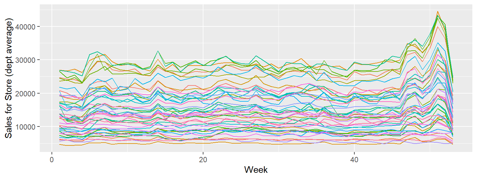
We have this

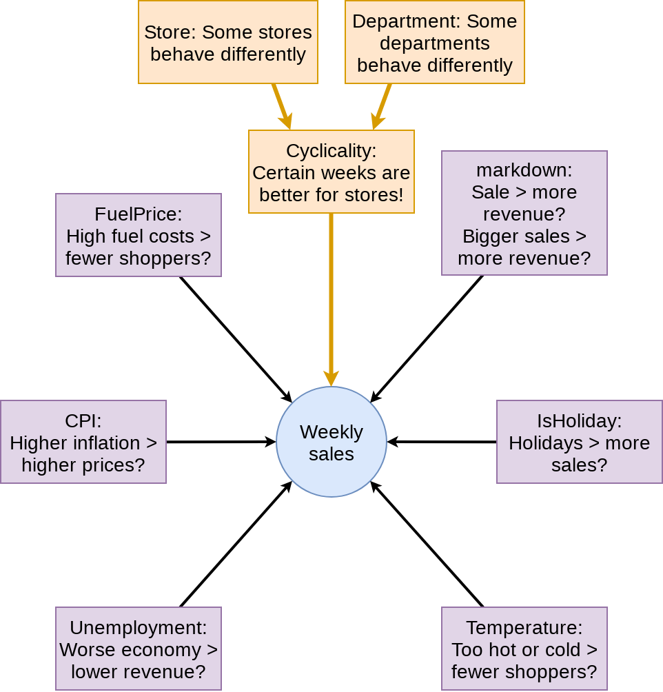
What to put in the model?

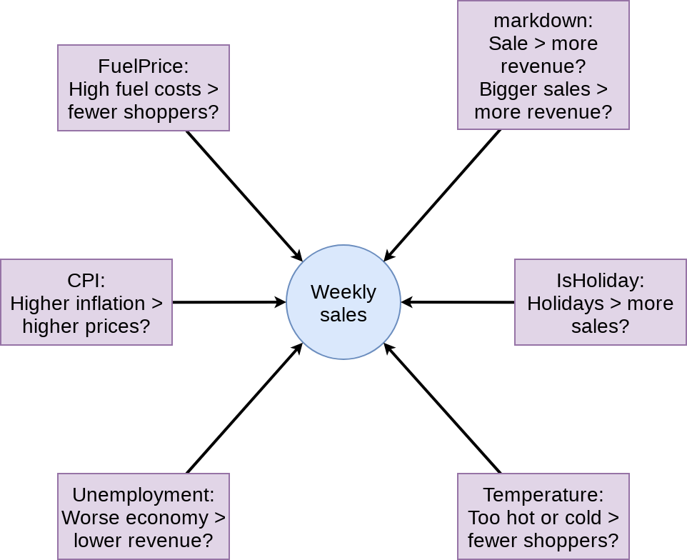
First model

mod1 <- lm(Weekly_mult ~ factor(IsHoliday) + factor(markdown>0) +
                         markdown + Temperature +
                         Fuel_Price + CPI + Unemployment,
           data=df)
tidy(mod1)

## # A tibble: 8 x 5
##   term                         estimate   std.error statistic   p.value
##   <chr>                           <dbl>       <dbl>     <dbl>     <dbl>
## 1 (Intercept)               1.24        0.0370         33.5   4.10e-245
## 2 factor(IsHoliday)TRUE     0.0868      0.0124          6.99  2.67e- 12
## 3 factor(markdown > 0)TRUE  0.0531      0.00885         6.00  2.00e-  9
## 4 markdown                  0.000000741 0.000000875     0.847 3.97e-  1
## 5 Temperature              -0.000763    0.000181       -4.23  2.38e-  5
## 6 Fuel_Price               -0.0706      0.00823        -8.58  9.90e- 18
## 7 CPI                      -0.0000837   0.0000887      -0.944 3.45e-  1
## 8 Unemployment              0.00410     0.00182         2.25  2.45e-  2

glance(mod1)

## # A tibble: 1 x 12
##   r.squared adj.r.squared sigma statistic  p.value    df   logLik     AIC    BIC
##       <dbl>         <dbl> <dbl>     <dbl>    <dbl> <dbl>    <dbl>   <dbl>  <dbl>
## 1  0.000481      0.000464  2.03      29.0 2.96e-40     7 -895684.  1.79e6 1.79e6
## # ... with 3 more variables: deviance <dbl>, df.residual <int>, nobs <int>

Prep submission and check in sample WMAE

# Out of sample result
df_test$Weekly_mult <- predict(mod1, df_test)
df_test$Weekly_Sales <- df_test$Weekly_mult * df_test$store_avg

# Required to submit a csv of Id and Weekly_Sales
write.csv(df_test[,c("Id","Weekly_Sales")],
          "WMT_linear.csv",
          row.names=FALSE)

# track
df_test$WS_linear <- df_test$Weekly_Sales

# Check in sample WMAE
df$WS_linear <- predict(mod1, df) * df$store_avg
w <- wmae(actual=df$Weekly_Sales, predicted=df$WS_linear, holidays=df$IsHoliday)
names(w) <- "Linear"
wmaes <- c(w)
wmaes

##  Linear 
## 3073.57

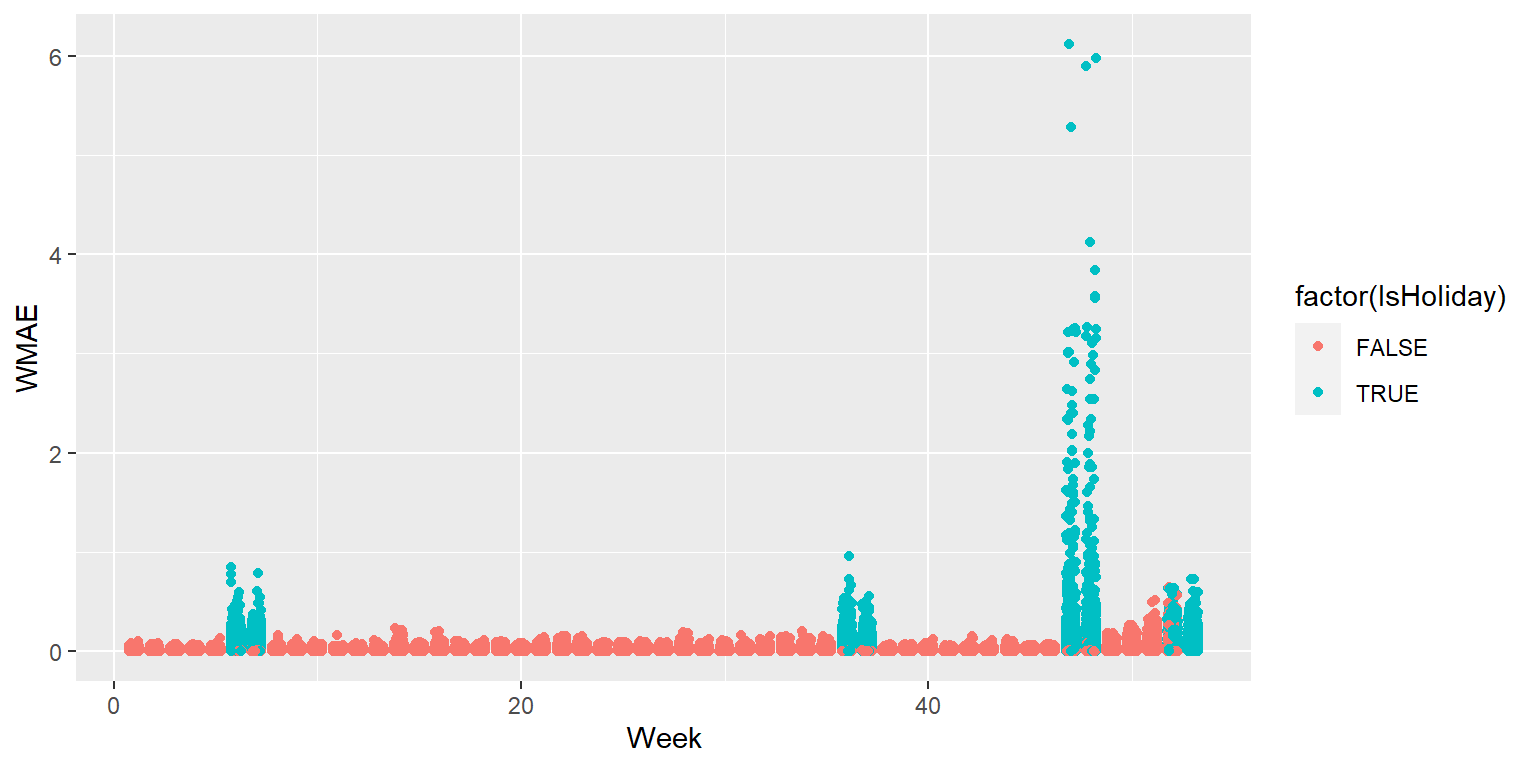
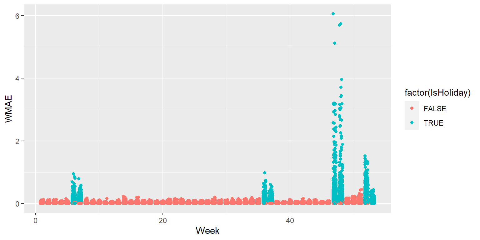
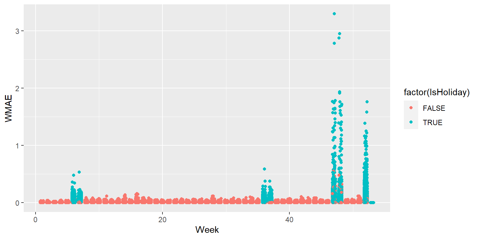
Visualizing in sample WMAE

wmae_obs <- function(actual, predicted, holidays) {
  abs(actual-predicted)*(holidays*5+1) / (length(actual) + 4*sum(holidays))
}
df$wmaes  <- wmae_obs(actual=df$Weekly_Sales, predicted=df$WS_linear,
                      holidays=df$IsHoliday)
ggplot(data=df, aes(y=wmaes, x=week, color=factor(IsHoliday))) + 
  geom_jitter(width=0.25) + xlab("Week") + ylab("WMAE")

Back to the drawing board…

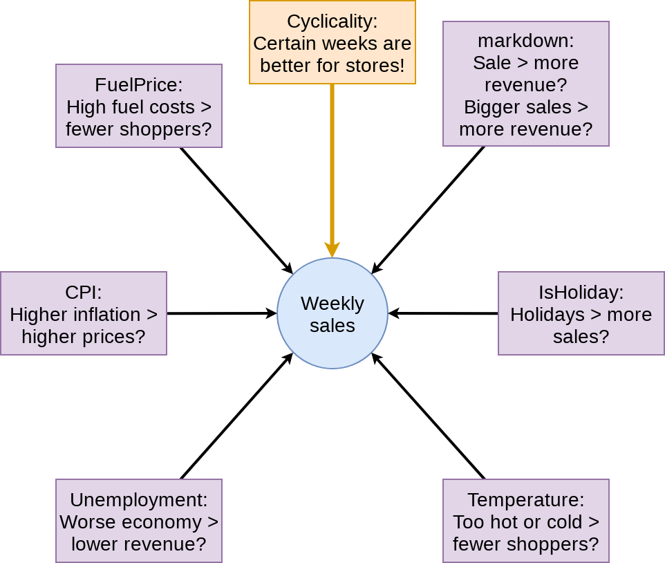
Second model: Including week

mod2 <- lm(Weekly_mult ~ factor(week) + factor(IsHoliday) + factor(markdown>0) +
                         markdown + Temperature +
                         Fuel_Price + CPI + Unemployment,
           data=df)
tidy(mod2)

## # A tibble: 60 x 5
##    term           estimate std.error statistic   p.value
##    <chr>             <dbl>     <dbl>     <dbl>     <dbl>
##  1 (Intercept)      1.00      0.0452     22.1  3.11e-108
##  2 factor(week)2   -0.0648    0.0372     -1.74 8.19e-  2
##  3 factor(week)3   -0.169     0.0373     -4.54 5.75e-  6
##  4 factor(week)4   -0.0716    0.0373     -1.92 5.47e-  2
##  5 factor(week)5    0.0544    0.0372      1.46 1.44e-  1
##  6 factor(week)6    0.161     0.0361      4.45 8.79e-  6
##  7 factor(week)7    0.265     0.0345      7.67 1.72e- 14
##  8 factor(week)8    0.109     0.0340      3.21 1.32e-  3
##  9 factor(week)9    0.0823    0.0340      2.42 1.55e-  2
## 10 factor(week)10   0.101     0.0341      2.96 3.04e-  3
## # ... with 50 more rows

glance(mod2)

## # A tibble: 1 x 12
##   r.squared adj.r.squared sigma statistic p.value    df   logLik     AIC     BIC
##       <dbl>         <dbl> <dbl>     <dbl>   <dbl> <dbl>    <dbl>   <dbl>   <dbl>
## 1   0.00501       0.00487  2.02      35.9       0    59 -894728.  1.79e6  1.79e6
## # ... with 3 more variables: deviance <dbl>, df.residual <int>, nobs <int>

Prep submission and check in sample WMAE

# Out of sample result
df_test$Weekly_mult <- predict(mod2, df_test)
df_test$Weekly_Sales <- df_test$Weekly_mult * df_test$store_avg

# Required to submit a csv of Id and Weekly_Sales
write.csv(df_test[,c("Id","Weekly_Sales")],
          "WMT_linear2.csv",
          row.names=FALSE)

# track
df_test$WS_linear2 <- df_test$Weekly_Sales

# Check in sample WMAE
df$WS_linear2 <- predict(mod2, df) * df$store_avg
w <- wmae(actual=df$Weekly_Sales, predicted=df$WS_linear2, holidays=df$IsHoliday)
names(w) <- "Linear 2"
wmaes <- c(wmaes, w)
wmaes

##   Linear Linear 2 
## 3073.570 3230.643

Visualizing in sample WMAE

df$wmaes  <- wmae_obs(actual=df$Weekly_Sales, predicted=df$WS_linear2,
                      holidays=df$IsHoliday)
ggplot(data=df, aes(y=wmaes,
                    x=week,
                    color=factor(IsHoliday))) + 
  geom_jitter(width=0.25) + xlab("Week") + ylab("WMAE")

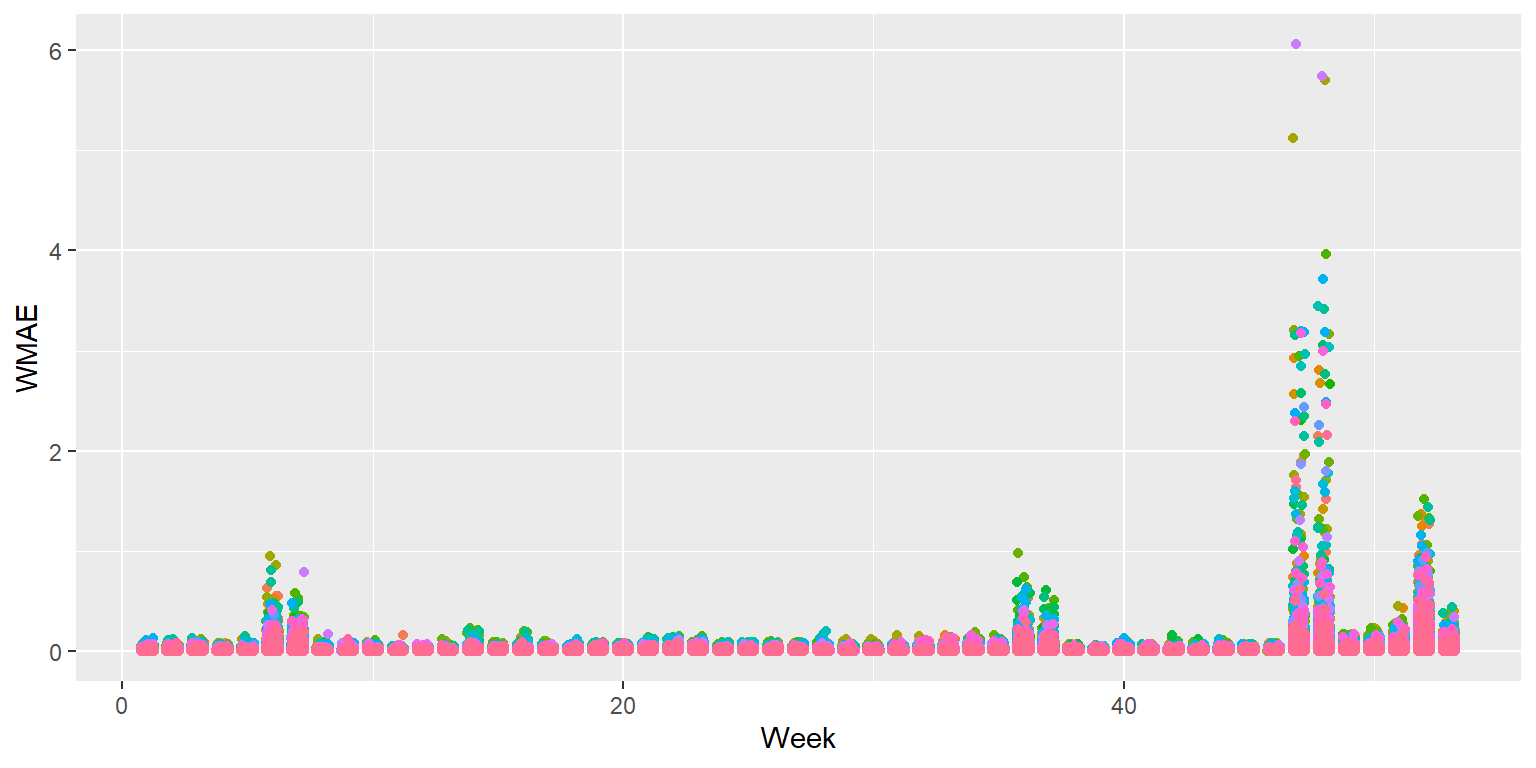
Visualizing in sample WMAE by Store

ggplot(data=df, aes(y=wmae_obs(actual=Weekly_Sales, predicted=WS_linear2,
                               holidays=IsHoliday),
                    x=week,
                    color=factor(Store))) + 
  geom_jitter(width=0.25) + xlab("Week") + ylab("WMAE") + 
  theme(legend.position="none")

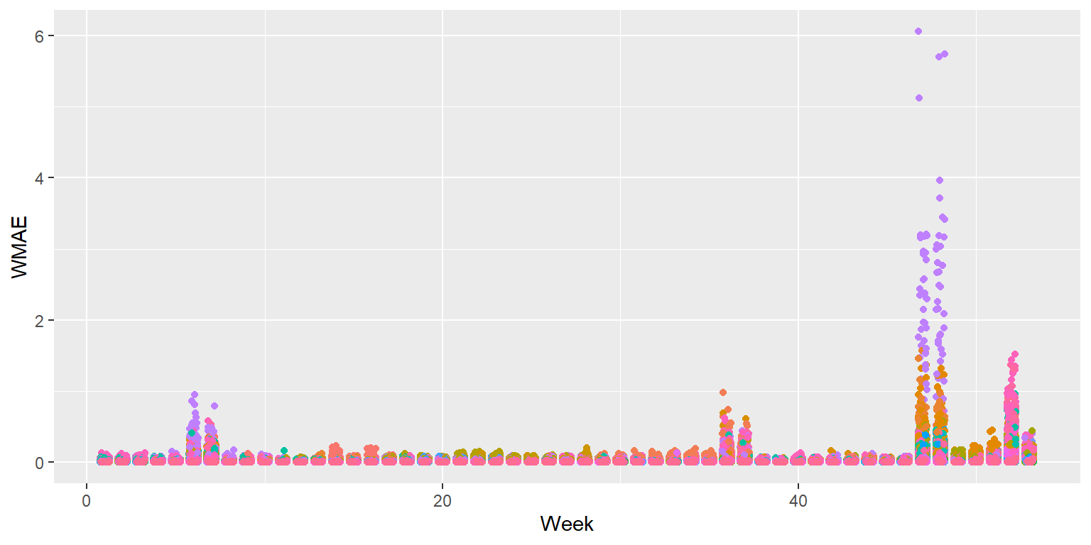
Visualizing in sample WMAE by Dept

ggplot(data=df, aes(y=wmae_obs(actual=Weekly_Sales, predicted=WS_linear2,
                               holidays=IsHoliday),
                    x=week,
                    color=factor(Dept))) + 
  geom_jitter(width=0.25) + xlab("Week") + ylab("WMAE") + 
  theme(legend.position="none")

Back to the drawing board…

Third model: Including week x Store x Dept

mod3 <- lm(Weekly_mult ~ factor(week):factor(Store):factor(Dept) + factor(IsHoliday) + factor(markdown>0) +
                         markdown + Temperature +
                         Fuel_Price + CPI + Unemployment,
           data=df)
## Error: cannot allocate vector of size 606.8Gb

…

Third model: Including week x Store x Dept

Use fixest’s feols() – it really is more efficient!

library(fixest)
mod3 <- feols(Weekly_mult ~ markdown +
            Temperature +
            Fuel_Price +
            CPI +
            Unemployment | id, data=df)
tidy(mod3)

## # A tibble: 5 x 5
##   term            estimate   std.error statistic  p.value
##   <chr>              <dbl>       <dbl>     <dbl>    <dbl>
## 1 markdown     -0.00000139 0.000000295     -4.73 2.24e- 6
## 2 Temperature   0.00135    0.000243         5.55 2.83e- 8
## 3 Fuel_Price   -0.0637     0.00905         -7.04 1.92e-12
## 4 CPI           0.00150    0.000800         1.87 6.13e- 2
## 5 Unemployment -0.0303     0.00386         -7.85 4.14e-15

glance(mod3)

## # A tibble: 1 x 9
##   r.squared adj.r.squared within.r.squared pseudo.r.squared sigma   nobs     AIC
##       <dbl>         <dbl>            <dbl>            <dbl> <dbl>  <int>   <dbl>
## 1     0.823         0.712         0.000540               NA  1.09 421564  1.39e6
## # ... with 2 more variables: BIC <dbl>, logLik <dbl>

Prep submission and check in sample WMAE

# Out of sample result
df_test$Weekly_mult <- predict(mod3, df_test)
df_test$Weekly_Sales <- df_test$Weekly_mult * df_test$store_avg
# Replace NA values with store average
df_test <- df_test %>%
  mutate(Weekly_Sales = ifelse(is.na(Weekly_Sales), naive_mean, Weekly_Sales))


# Required to submit a csv of Id and Weekly_Sales
write.csv(df_test[,c("Id","Weekly_Sales")],
          "WMT_FE.csv",
          row.names=FALSE)

# track
df_test$WS_FE <- df_test$Weekly_Sales

# Check in sample WMAE
df$WS_FE <- predict(mod3, df) * df$store_avg
w <- wmae(actual=df$Weekly_Sales, predicted=df$WS_FE, holidays=df$IsHoliday)
names(w) <- "FE"
wmaes <- c(wmaes, w)
wmaes

##   Linear Linear 2       FE 
## 3073.570 3230.643 1552.190

Visualizing in sample WMAE

df$wmaes  <- wmae_obs(actual=df$Weekly_Sales, predicted=df$WS_FE,
                      holidays=df$IsHoliday)
ggplot(data=df, aes(y=wmaes,
                    x=week,
                    color=factor(IsHoliday))) + 
  geom_jitter(width=0.25) + xlab("Week") + ylab("WMAE")

## Warning: Removed 6 rows containing missing values (geom_point).

Maybe the data is part of the problem?

What problems might there be for our testing sample?
- What is different from testing to training?
Can we fix them?
- If so, how?

This was a real problem!

Walmart provided this data back in 2014 as part of a recruiting exercise
This is what the group project will be like
- 4 to 5 group members tackling a real life data problem
- You will have training data but testing data will be withheld
- Submit on Kaggle

Project deliverables

Kaggle submission
Your code for your submission, walking through what you did
A 15 minute presentation on the last day of class describing:
- Your approach
A report discussing
- Main points and findings
- Exploratory analysis of the data used
- Your model development, selection, implementation, evaluation, and refinement
- A conclusion on how well your group did and what you learned in the process

ACCT 420: Project Example

Project Example

Dr. Richard M. Crowleyrcrowley@smu.edu.sghttp://rmc.link/

Weekly revenue prediction at Walmart

The question

More specifically…

The data

Walmart’s evaluation metric

Before we get started…

Also…

Load data and packages

Cleaning

What this looks like

Cleaning: Missing CPI and Unemployment

Cleaning: Adding IDs

What the IDs look like

Add in (store, department) average sales

Add in (week, store, dept) average sales

ISSUE: New (week, store, dept) groups

Cleaning is done

Tackling the problem

First try

What to put in the model?

First model

Prep submission and check in sample WMAE

Visualizing in sample WMAE

Back to the drawing board…

Second model: Including week

Prep submission and check in sample WMAE

Visualizing in sample WMAE

Visualizing in sample WMAE by Store

Visualizing in sample WMAE by Dept

Back to the drawing board…

Third model: Including week x Store x Dept

Third model: Including week x Store x Dept

Prep submission and check in sample WMAE

Visualizing in sample WMAE

Maybe the data is part of the problem?

End Matter

This was a real problem!

Project deliverables

Packages used for these slides

Dr. Richard M. Crowley
rcrowley@smu.edu.sg
http://rmc.link/