ACCT 420: Project example

Dr. Richard M. Crowley

rcrowley@smu.edu.sg

https://rmc.link/

Weekly revenue prediction at Walmart

The question

How can we predict weekly departmental revenue for Walmart, leveraging our knowledge of Walmart, its business, and some limited historical information?

• Predict weekly for 115,064 (Store, Department, Week) tuples
  • From 2012-11-02 to 2013-07-26
• Using [incomplete] weekly revenue data from 2010-02-015 to 2012-10-26
  • By department
    • Some weeks missing for some departments

This is a real problem posed by Walmart

As such, the data is messy to work with. Real data is rarely clean.

More specifically…

• Consider time dimensions
  • What matters:
    • Time of the year?
    • Holidays?
    • Do different stores or departments behave differently?
• Wrinkles:
  • Walmart won’t give us testing data
    • But they’ll tell us how well the algorithm performs
  • We can’t use past week sales for prediction because we won’t have it for most of the prediction…

The data

• Revenue by week for each department of each of 45 stores
  • Department is just a number between 1 and 99
    • We don’t know what these numbers mean
  • Date of that week
  • If the week is considered a holiday for sales purposes
    • Super Bowl, Labor Day, Black Friday, Christmas
• Store data:
  • Which store the data is for, 1 to 45
  • Store type (A, B, or C)
    • We don’t know what these letters mean
  • Store size
• Other data, by week and location:
  • Temperature, gas price, sales (by department), CPI, Unemployment rate, Holidays

Walmart’s evaluation metric

• Walmart uses MAE (mean absolute error), but with a twist:
  • They care more about holidays, so any error on holidays has 5 times the penalty
  • They call this WMAE, for weighted mean absolute error

\[ WMAE = \frac{1}{\sum w_i} \sum_{i=1}^{n} w_i \left|y_i-\hat{y}_i\right| \]

• \(n\) is the number of test data points
• \(\hat{y}_i\) is your prediction
• \(y_i\) is the actual sales
• \(w_i\) is 5 on holidays and 1 otherwise

wmae <- function(actual, predicted, holidays) {
  ids <- !is.na(actual) & !is.na(predicted) & !is.na(holidays)
  sum(abs(actual[ids]-predicted[ids])*(holidays[ids]*4+1)) /(length(actual[ids]) + 4*sum(holidays[ids]))
}

Before we get started…

• The data isn’t very clean:
  • Markdowns are given by 5 separate variables instead of 1
  • Date is text format instead of a date
  • CPI and unemployment data are missing in around a third of the testing data
  • There are some (week, store, department) groups missing from our training data!

We’ll have to fix these

Also…

• Some features to add:
  • Year
  • Week
  • A unique ID for tracking (week, firm, department) tuples
  • The ID Walmart requests we use for submissions
  • Average sales by (store, department)
  • Average sales by (week, store, department)

Load data and packages

library(tidyverse)  # We'll extensively use dplyr here
library(lubridate)  # Great for simple date functions
library(broom)      # To view results in a tidy manner
weekly <- read_csv("../../Data/WMT_train.csv")
weekly.test <- read_csv("../../Data/WMT_test.csv")
weekly.features <- read_csv("../../Data/WMT_features.csv")
weekly.stores <- read_csv("../../Data/WMT_stores.csv")

• weekly is our training data
• weekly.test is our testing data – no Weekly_Sales column
• weekly.features is general information about (week, store) pairs
  • Temperature, pricing, etc.
• weekly.stores is general information about each store

Cleaning

preprocess_data <- function(df) {
  # Merge the data together (Pulled from outside of function -- "scoping")
  df <- inner_join(df, weekly.stores)
  df <- inner_join(df, weekly.features[,1:11])
  # Compress the weird markdown information to 1 variable
  df$markdown <- 0
  df[!is.na(df$MarkDown1),]$markdown <- df[!is.na(df$MarkDown1),]$MarkDown1
  df[!is.na(df$MarkDown2),]$markdown <- df[!is.na(df$MarkDown2),]$MarkDown2
  df[!is.na(df$MarkDown3),]$markdown <- df[!is.na(df$MarkDown3),]$MarkDown3
  df[!is.na(df$MarkDown4),]$markdown <- df[!is.na(df$MarkDown4),]$MarkDown4
  df[!is.na(df$MarkDown5),]$markdown <- df[!is.na(df$MarkDown5),]$MarkDown5
  # Fix dates and add useful time variables
  df$date <- as.Date(df$Date)
  df$week <- week(df$date)
  df$year <- year(df$date)
  # Output the data
  df
}

df <- preprocess_data(weekly)
df_test <- preprocess_data(weekly.test)

Merge data, fix markdown, build time data

What this looks like

df[91:94,] %>%
  select(Store, date, markdown, MarkDown3, MarkDown4, MarkDown5) %>%
  html_df()

Store	date	markdown	MarkDown3	MarkDown4	MarkDown5
1	2011-10-28	0.00	NA	NA	NA
1	2011-11-04	0.00	NA	NA	NA
1	2011-11-11	6551.42	215.07	2406.62	6551.42
1	2011-11-18	5988.57	51.98	427.39	5988.57

df[1:2,] %>% select(date, week, year) %>% html_df()

date	week	year
2010-02-05	6	2010
2010-02-12	7	2010

Cleaning: Missing CPI and Unemployment

# Fill in missing CPI and Unemployment data
df_test <- df_test %>%
  group_by(Store, year) %>%
  mutate(CPI=ifelse(is.na(CPI), mean(CPI,na.rm=T), CPI),
         Unemployment=ifelse(is.na(Unemployment),
                             mean(Unemployment,na.rm=T),
                             Unemployment)) %>%
  ungroup()

Apply the (year, Store)’s CPI and Unemployment to missing data

Cleaning: Adding IDs

• Build a unique ID
  • Since Store, week, and department are all 2 digits, make a 6 digit number with 2 digits for each
    • sswwdd
• Build Walmart’s requested ID for submissions
  • ss_dd_YYYY-MM-DD

# Unique IDs in the data for tracking across data
df$id <- df$Store *10000 + df$week * 100 + df$Dept
df_test$id <- df_test$Store *10000 + df_test$week * 100 + df_test$Dept

# Id needed for submission
df_test$Id <- paste0(df_test$Store,'_',df_test$Dept,"_",df_test$date)

What the IDs look like

html_df(df_test[c(20000,40000,60000),c("Store","week","Dept","id","Id")])

Store	week	Dept	id	Id
8	27	33	82733	8_33_2013-07-05
15	46	91	154691	15_91_2012-11-16
23	52	25	235225	23_25_2012-12-28

Add in (store, department) average sales

# Calculate average by store-dept and distribute to df_test
df <- df %>%
  group_by(Store, Dept) %>% 
  mutate(store_avg=mean(Weekly_Sales, rm.na=T)) %>%
  ungroup()
df_sa <- df %>%
  group_by(Store, Dept) %>%
  slice(1) %>%
  select(Store, Dept, store_avg) %>%
  ungroup()
df_test <- left_join(df_test, df_sa)
# 36 observations have invalid department codes -- ignore (set to 0)
df_test[is.na(df_test$store_avg),]$store_avg  <- 0

# Calculate multipliers based on store_avg (and removing NaN and Inf)
df$Weekly_mult <- df$Weekly_Sales / df$store_avg
df[!is.finite(df$Weekly_mult),]$Weekly_mult <- NA

Add in (week, store, dept) average sales

# Calculate mean by week-store-dept and distribute to df_test
df <- df %>%
  group_by(Store, Dept, week) %>%
  mutate(naive_mean=mean(Weekly_Sales, rm.na=T)) %>%
  ungroup()
df_wm <- df %>%
  group_by(Store, Dept, week) %>%
  slice(1) %>%
  ungroup() %>%
  select(Store, Dept, week, naive_mean)
df_test <- df_test %>% arrange(Store, Dept, week)
df_test <- left_join(df_test, df_wm)

ISSUE: New (week, store, dept) groups

• This is in our testing data!
  • So we’ll need to predict out groups we haven’t observed at all

table(is.na(df_test$naive_mean))

 FALSE   TRUE 
113827   1237 

• Fix: Fill with 1 or 2 lags where possible using ifelse() and lag()
• Fix: Fill with 1 or 2 leads where possible using ifelse() and lag()
• Fill with store_avg when the above fail
• Code is available in the code file – a bunch of code like:

df_test <- df_test %>%
  arrange(Store, Dept, date) %>%
  group_by(Store, Dept) %>%
  mutate(naive_mean=ifelse(is.na(naive_mean), lag(naive_mean),naive_mean)) %>%
  ungroup()

Cleaning is done

• Data is in order
  • No missing values where data is needed
  • Needed values created

df %>% 
  group_by(week, Store) %>%
  mutate(sales=mean(Weekly_Sales)) %>%
  slice(1) %>%
  ungroup() %>%
  ggplot(aes(y=sales, x=week, color=factor(Store))) +
  geom_line() + xlab("Week") + ylab("Sales for Store (dept average)") + 
  theme(legend.position="none")

Tackling the problem

First try

• Ideal: Use last week to predict next week!

No data for testing…

• First instinct: try to use a linear regression to solve this

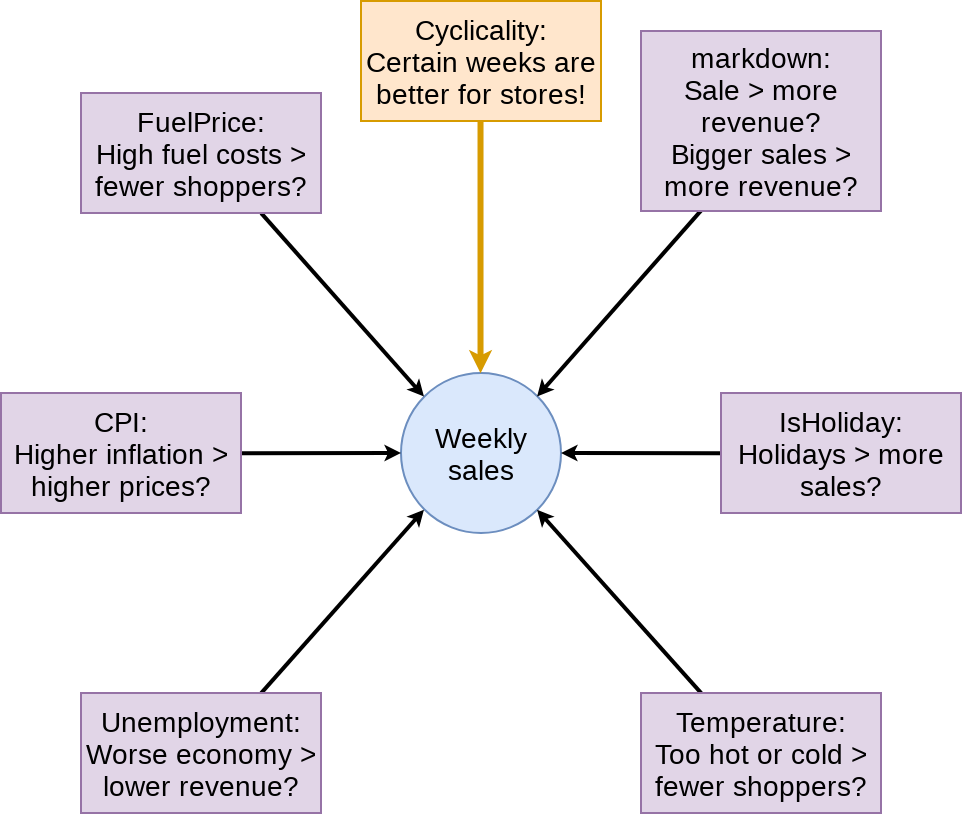
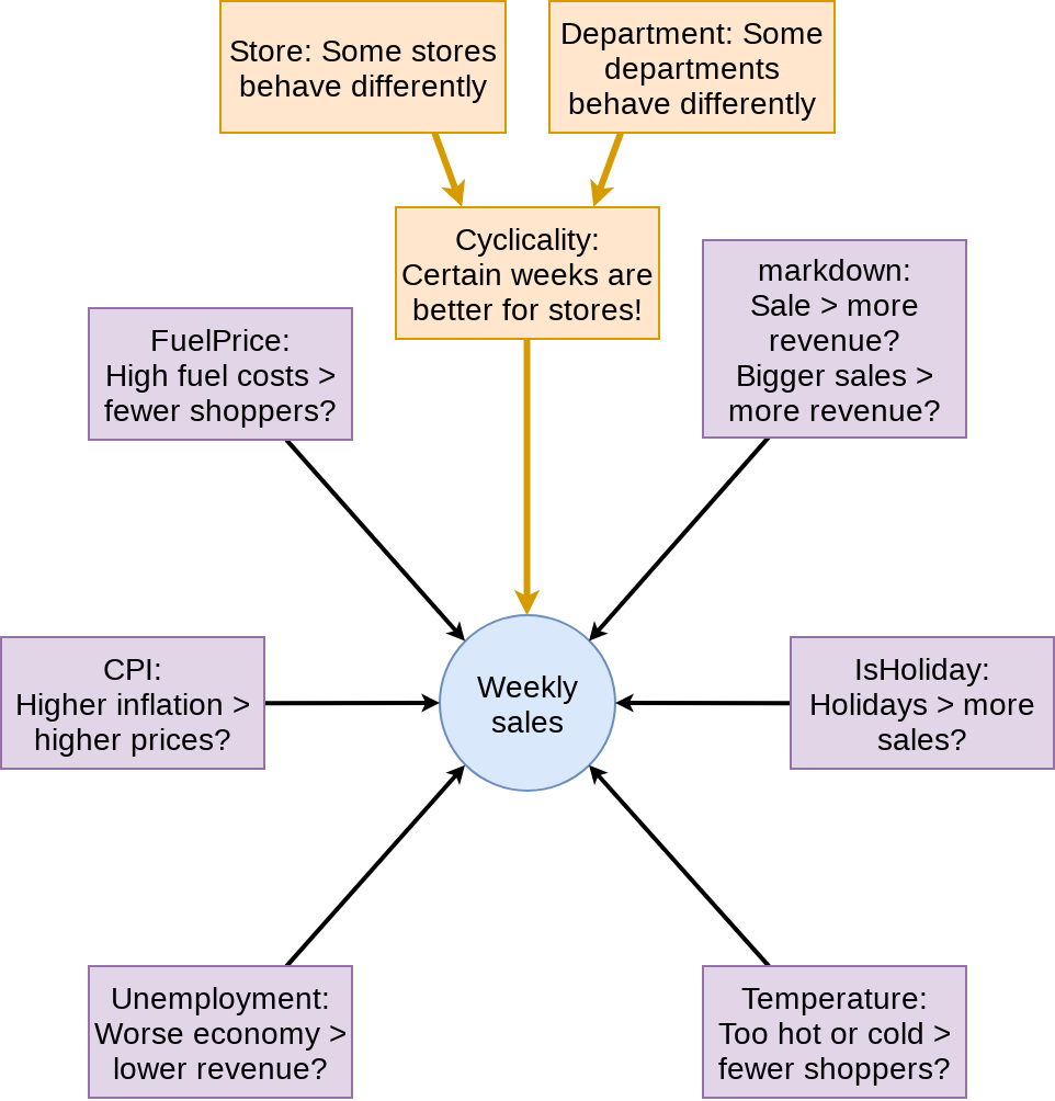
We have this

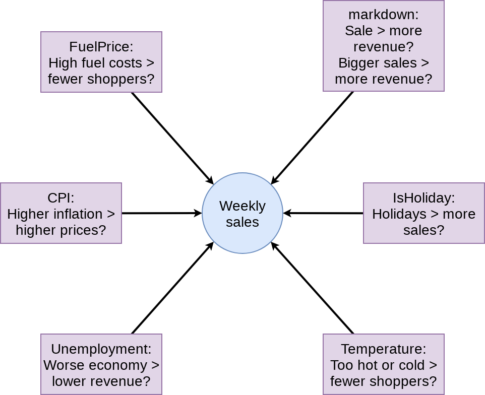
What to put in the model?

First model

mod1 <- lm(Weekly_mult ~ factor(IsHoliday) + factor(markdown>0) +
                         markdown + Temperature +
                         Fuel_Price + CPI + Unemployment,
           data=df)
tidy(mod1)

# A tibble: 8 × 5
  term                         estimate   std.error statistic   p.value
  <chr>                           <dbl>       <dbl>     <dbl>     <dbl>
1 (Intercept)               1.24        0.0370         33.5   4.10e-245
2 factor(IsHoliday)TRUE     0.0868      0.0124          6.99  2.67e- 12
3 factor(markdown > 0)TRUE  0.0531      0.00885         6.00  2.00e-  9
4 markdown                  0.000000741 0.000000875     0.847 3.97e-  1
5 Temperature              -0.000763    0.000181       -4.23  2.38e-  5
6 Fuel_Price               -0.0706      0.00823        -8.58  9.90e- 18
7 CPI                      -0.0000837   0.0000887      -0.944 3.45e-  1
8 Unemployment              0.00410     0.00182         2.25  2.45e-  2

glance(mod1)

# A tibble: 1 × 12
  r.squared adj.r.squared sigma statistic  p.value    df   logLik     AIC    BIC
      <dbl>         <dbl> <dbl>     <dbl>    <dbl> <dbl>    <dbl>   <dbl>  <dbl>
1  0.000481      0.000464  2.03      29.0 2.96e-40     7 -895684.  1.79e6 1.79e6
# … with 3 more variables: deviance <dbl>, df.residual <int>, nobs <int>

Prep submission and check in sample WMAE

# Out of sample result
df_test$Weekly_mult <- predict(mod1, df_test)
df_test$Weekly_Sales <- df_test$Weekly_mult * df_test$store_avg

# Required to submit a csv of Id and Weekly_Sales
write.csv(df_test[,c("Id","Weekly_Sales")],
          "WMT_linear.csv",
          row.names=FALSE)

# track
df_test$WS_linear <- df_test$Weekly_Sales

# Check in sample WMAE
df$WS_linear <- predict(mod1, df) * df$store_avg
w <- wmae(actual=df$Weekly_Sales, predicted=df$WS_linear, holidays=df$IsHoliday)
names(w) <- "Linear"
wmaes <- c(w)
wmaes

 Linear 
3073.57 

Performance for linear model

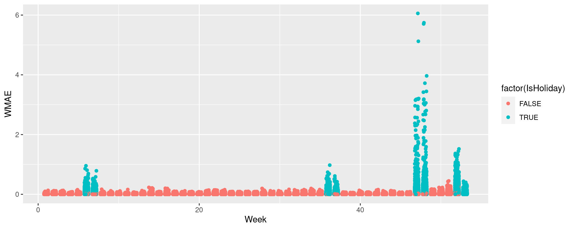
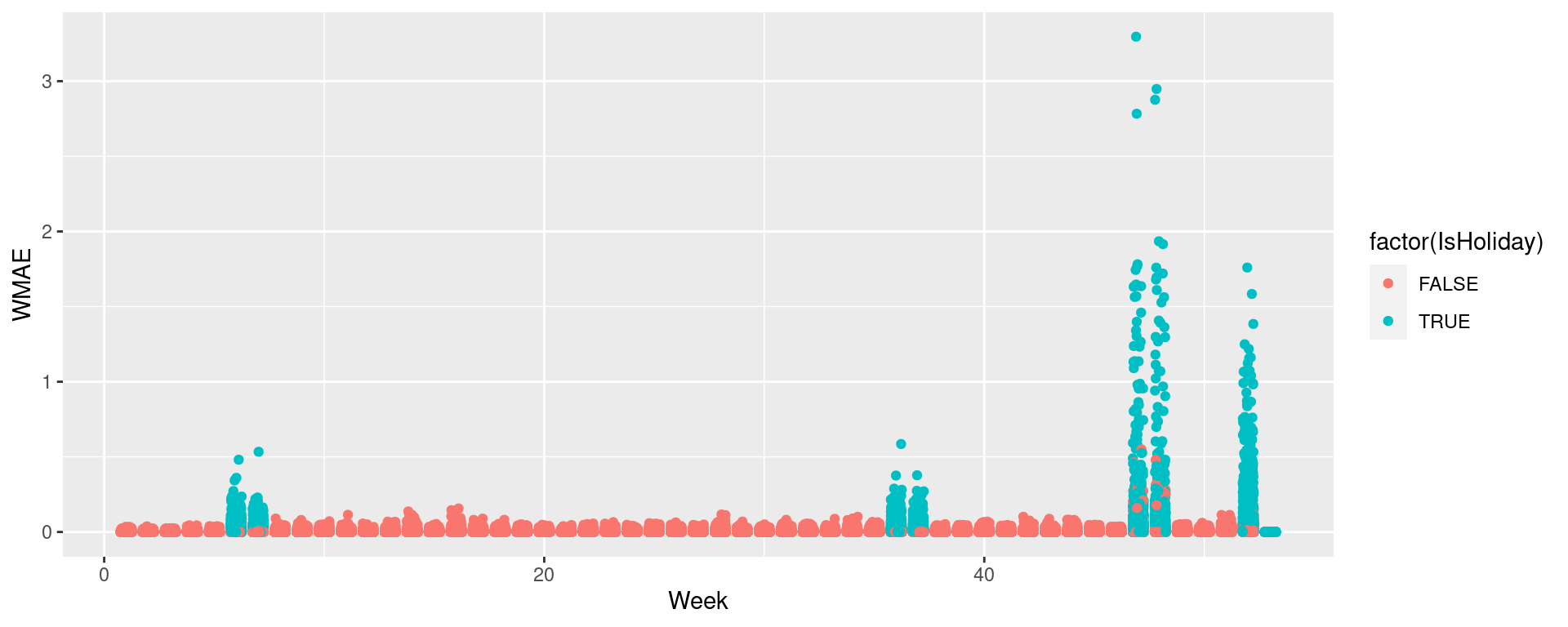
Visualizing in sample WMAE

wmae_obs <- function(actual, predicted, holidays) {
  abs(actual-predicted)*(holidays*5+1) / (length(actual) + 4*sum(holidays))
}
df$wmaes  <- wmae_obs(actual=df$Weekly_Sales, predicted=df$WS_linear,
                      holidays=df$IsHoliday)
ggplot(data=df, aes(y=wmaes, x=week, color=factor(IsHoliday))) + 
  geom_jitter(width=0.25) + xlab("Week") + ylab("WMAE")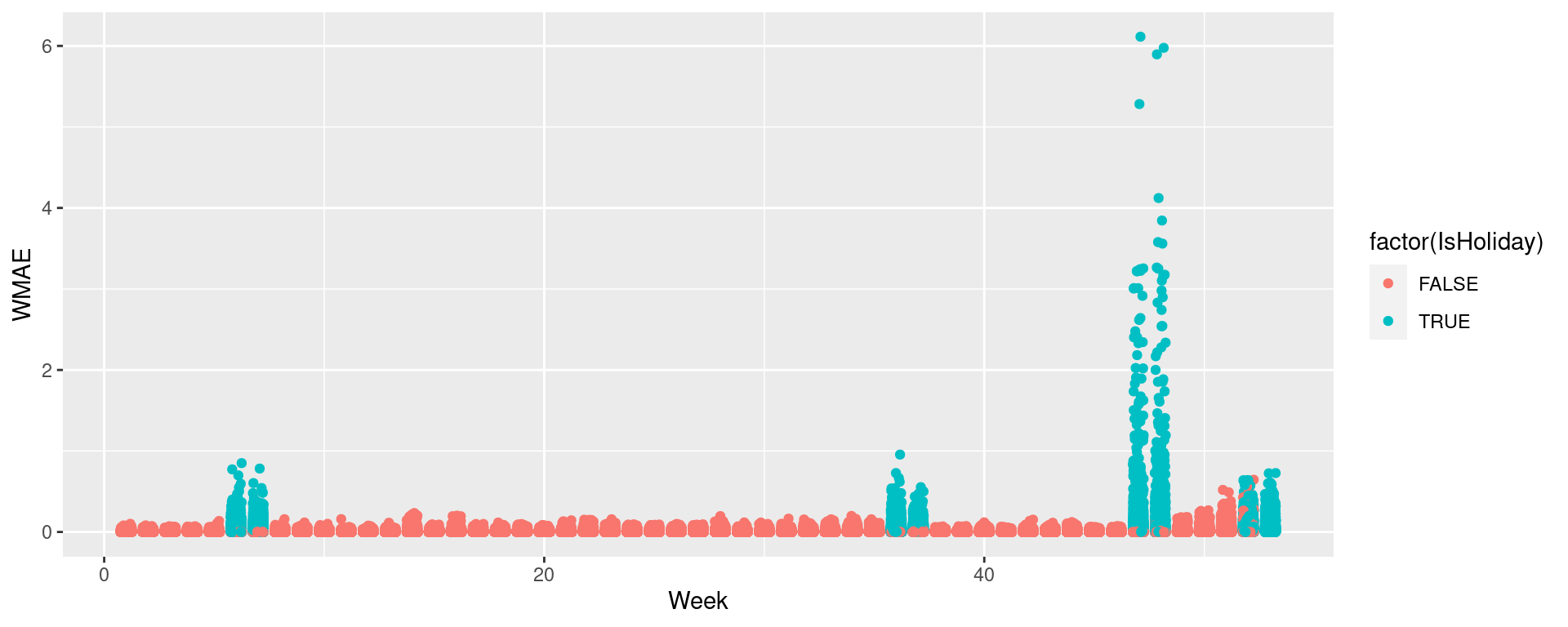

Back to the drawing board…

Second model: Including week

mod2 <- lm(Weekly_mult ~ factor(week) + factor(IsHoliday) + factor(markdown>0) +
                         markdown + Temperature +
                         Fuel_Price + CPI + Unemployment,
           data=df)
tidy(mod2)

# A tibble: 60 × 5
   term           estimate std.error statistic   p.value
   <chr>             <dbl>     <dbl>     <dbl>     <dbl>
 1 (Intercept)      1.00      0.0452     22.1  3.11e-108
 2 factor(week)2   -0.0648    0.0372     -1.74 8.19e-  2
 3 factor(week)3   -0.169     0.0373     -4.54 5.75e-  6
 4 factor(week)4   -0.0716    0.0373     -1.92 5.47e-  2
 5 factor(week)5    0.0544    0.0372      1.46 1.44e-  1
 6 factor(week)6    0.161     0.0361      4.45 8.79e-  6
 7 factor(week)7    0.265     0.0345      7.67 1.72e- 14
 8 factor(week)8    0.109     0.0340      3.21 1.32e-  3
 9 factor(week)9    0.0823    0.0340      2.42 1.55e-  2
10 factor(week)10   0.101     0.0341      2.96 3.04e-  3
# … with 50 more rows

glance(mod2)

# A tibble: 1 × 12
  r.squared adj.r.squared sigma statistic p.value    df   logLik      AIC    BIC
      <dbl>         <dbl> <dbl>     <dbl>   <dbl> <dbl>    <dbl>    <dbl>  <dbl>
1   0.00501       0.00487  2.02      35.9       0    59 -894728. 1789577. 1.79e6
# … with 3 more variables: deviance <dbl>, df.residual <int>, nobs <int>

Prep submission and check in sample WMAE

# Out of sample result
df_test$Weekly_mult <- predict(mod2, df_test)
df_test$Weekly_Sales <- df_test$Weekly_mult * df_test$store_avg

# Required to submit a csv of Id and Weekly_Sales
write.csv(df_test[,c("Id","Weekly_Sales")],
          "WMT_linear2.csv",
          row.names=FALSE)

# track
df_test$WS_linear2 <- df_test$Weekly_Sales

# Check in sample WMAE
df$WS_linear2 <- predict(mod2, df) * df$store_avg
w <- wmae(actual=df$Weekly_Sales, predicted=df$WS_linear2, holidays=df$IsHoliday)
names(w) <- "Linear 2"
wmaes <- c(wmaes, w)
wmaes

  Linear Linear 2 
3073.570 3230.643 

Performance for linear model 2

wmaes_out

  Linear Linear 2 
  4993.4   5618.4 

Visualizing in sample WMAE

df$wmaes  <- wmae_obs(actual=df$Weekly_Sales, predicted=df$WS_linear2,
                      holidays=df$IsHoliday)
ggplot(data=df, aes(y=wmaes,
                    x=week,
                    color=factor(IsHoliday))) + 
  geom_jitter(width=0.25) + xlab("Week") + ylab("WMAE")

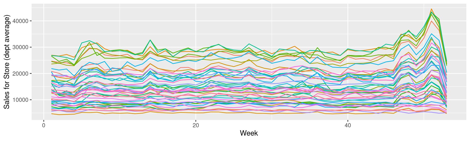
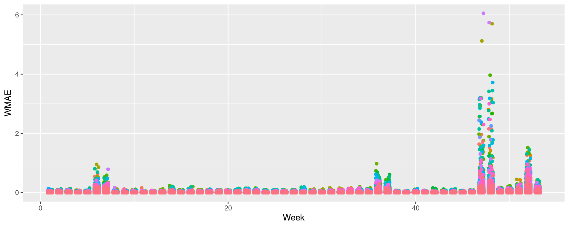
Visualizing in sample WMAE by Store

ggplot(data=df, aes(y=wmae_obs(actual=Weekly_Sales, predicted=WS_linear2,
                               holidays=IsHoliday),
                    x=week,
                    color=factor(Store))) + 
  geom_jitter(width=0.25) + xlab("Week") + ylab("WMAE") + 
  theme(legend.position="none")

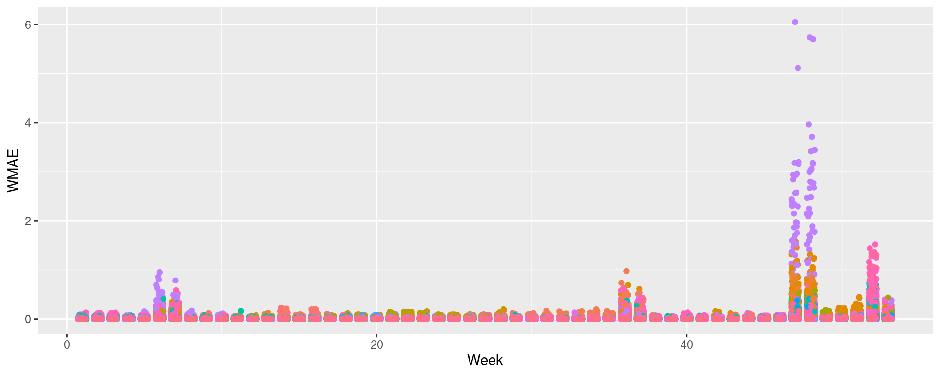
Visualizing in sample WMAE by Dept

ggplot(data=df, aes(y=wmae_obs(actual=Weekly_Sales, predicted=WS_linear2,
                               holidays=IsHoliday),
                    x=week,
                    color=factor(Dept))) + 
  geom_jitter(width=0.25) + xlab("Week") + ylab("WMAE") + 
  theme(legend.position="none")

Back to the drawing board…

Third model: Including week x Store x Dept

mod3 <- lm(Weekly_mult ~ factor(week):factor(Store):factor(Dept) + factor(IsHoliday) + factor(markdown>0) +
                         markdown + Temperature +
                         Fuel_Price + CPI + Unemployment,
           data=df)
## Error: cannot allocate vector of size 606.8Gb

…

Third model: Including week x Store x Dept

• Use fixest’s feols() – it really is more efficient!

library(fixest)
mod3 <- feols(Weekly_mult ~ markdown +
            Temperature +
            Fuel_Price +
            CPI +
            Unemployment | id, data=df)
tidy(mod3)

# A tibble: 5 × 5
  term            estimate   std.error statistic  p.value
  <chr>              <dbl>       <dbl>     <dbl>    <dbl>
1 markdown     -0.00000139 0.000000295     -4.73 2.24e- 6
2 Temperature   0.00135    0.000243         5.55 2.83e- 8
3 Fuel_Price   -0.0637     0.00905         -7.04 1.92e-12
4 CPI           0.00150    0.000800         1.87 6.13e- 2
5 Unemployment -0.0303     0.00386         -7.85 4.14e-15

glance(mod3)

# A tibble: 1 × 9
  r.squared adj.r.squared within.r.squared pseudo.r.squared sigma   nobs     AIC
      <dbl>         <dbl>            <dbl>            <dbl> <dbl>  <int>   <dbl>
1     0.823         0.712         0.000540               NA  1.09 421564  1.39e6
# … with 2 more variables: BIC <dbl>, logLik <dbl>

Prep submission and check in sample WMAE

# Out of sample result
df_test$Weekly_mult <- predict(mod3, df_test)
df_test$Weekly_Sales <- df_test$Weekly_mult * df_test$store_avg
# Replace NA values with store average
df_test <- df_test %>%
  mutate(Weekly_Sales = ifelse(is.na(Weekly_Sales), naive_mean, Weekly_Sales))

# Required to submit a csv of Id and Weekly_Sales
write.csv(df_test[,c("Id","Weekly_Sales")],
          "WMT_FE.csv",
          row.names=FALSE)

# track
df_test$WS_FE <- df_test$Weekly_Sales

# Check in sample WMAE
df$WS_FE <- predict(mod3, df) * df$store_avg
w <- wmae(actual=df$Weekly_Sales, predicted=df$WS_FE, holidays=df$IsHoliday)
names(w) <- "FE"
wmaes <- c(wmaes, w)
wmaes

  Linear Linear 2       FE 
3073.570 3230.643 1552.190 

Performance for FE model

wmaes_out

  Linear Linear 2       FE 
  4993.4   5618.4   3379.3 

Visualizing in sample WMAE

df$wmaes  <- wmae_obs(actual=df$Weekly_Sales, predicted=df$WS_FE,
                      holidays=df$IsHoliday)
ggplot(data=df, aes(y=wmaes,
                    x=week,
                    color=factor(IsHoliday))) + 
  geom_jitter(width=0.25) + xlab("Week") + ylab("WMAE")

Maybe the data is part of the problem?

• What problems might there be for our testing sample?
  • What is different from testing to training?
• Can we fix them?
  • If so, how?

Problems with the data

1. The holidays are not always on the same week
   • The Super Bowl is in weeks 6, 6, 7, 6
   • Labor day isn’t in our testing data at all!
   • Black Friday is in weeks 48, 47, and 47
   • Christmas is in weeks 53, 52, and 52
   • Manually adjust the data for these differences
2. Yearly growth – we aren’t capturing it, since we have such a small time span
   • We can manually adjust the data for this

Code is in the code file – a lot of dplyr

Performance overall

wmaes_out

    Linear   Linear 2         FE Shifted FE 
    4993.4     5618.4     3378.8     3274.8 

End Matter

This was a real problem!

• Walmart provided this data back in 2014 as part of a recruiting exercise
  • Details here
  • Discussion of first place entry
    • Code for first place entry
  • Discussion of second place entry
• This is what the group project will be like
  • 4 to 5 group members tackling a real life data problem
  • You will have training data but testing data will be withheld
  • Submit on Kaggle

Project deliverables

1. Kaggle submission
2. Your code for your submission, walking through what you did
3. A 15 minute presentation on the last day of class describing:
   • Your approach
4. A report discussing
   • Main points and findings
   • Exploratory analysis of the data used
   • Your model development, selection, implementation, evaluation, and refinement
   • A conclusion on how well your group did and what you learned in the process

Packages used for these slides

• broom
• DT
• downlit
• fixest
• kableExtra
• knitr
• lubridate
• quarto
• revealjs
• tidyverse

NOTES