ACCT 420: Course Logistics + R Refresh


Session 1


Dr. Richard M. Crowley

http://rmc.link/

About Me

Teaching

  • Sixth year at SMU
  • Teaching:
    • ACCT 101, Financial Accounting
    • ACCT 420, Forecasting and Forensic Analytics
    • ACCT 703, Analytical Methods in Accounting
    • IDIS 700, Machine Learning for Social Science
  • Before SMU: Taught at the University of Illinois Urbana-Champaign while completing my PhD

Research

  • Accounting disclosure: What companies say, and why it matters
    • Focus on social media and regulatory filing
  • Approach this using AI/ML techniques

Research highlights

  1. An advanced model for detecting financial misreporting using the text of annual reports.
  2. Multiple projects on Twitter showcasing:
    1. How companies are more likely to disclose both good and bad information than what is normal or expected
    2. That CSR disclosure on Twitter is not credible
    3. That executives’ disclosures are as important on Twitter as their firms’ disclosures
  3. Newer work on
    • COVID-19 reactions worldwide
    • Sentiment in accounting text
    • Space commercialization
    • Misinformation laws (e.g., POFMA)

The above all use some sort of Neural Network or text analytics approach.

About this course

What will this course cover?

  1. Foundations (today)
    • Thinking about analytics
    • In class: Setting a foundation for the course
    • Outside: Practice and refining skills on Datacamp
      • Pick any R course, any level, and try it out!
  2. Financial forecasting
    • Predict financial outcomes
    • Linear models

Getting familiar with forecasting using real data and R

What will this course cover?

  1. Binary classification
    • Event prediction
      • Shipping delays
      • Bankruptcy
    • Classification & detection
  2. Advanced methods
    • Non-numeric data (text)
    • Clustering
    • AI/Machine learning (ML)
      • 1 week on Ethics of AI
      • 2 weeks on current developments

Higher level financial forecasting, detection, and AI/ML

Datacamp

  • Datacamp is providing free access to their full library of analytics and coding online tutorials
    • You will have free access for 6 months (Usually $25 USD/mo)
  • Online tutorials include short exercises and videos to help you learn R
  • I have assigned some limited materials via a Datacamp class
    • These count towards participation
    • Sign up through the link on eLearn!
    • Datacamp automatically records when you finish these
    • I have personally done any tutorial I assign to ensure its quality
  • You are encouraged to go beyond the assigned materials – these will help you learn more about R and how to use it

Datacamp’s tutorials teach R from the ground up, and are mandatory unless you can already code in R.

Textbook

  • There is no required textbook
    • Datacamp is taking the place of the textbook
  • If you prefer having a textbook…

  • Other course materials (slides and articles) are available at:
  • Announcements will be only on eLearn

Teaching philosphy

  1. Analytics is best learned by doing it
    • Less lecture, more thinking
  2. Working with others greatly extends learning
    • If you are ahead:
      • The best sign that you’ve mastered a topic is if you can explain it to others
    • If you are lost:
      • Gives you a chance to get help the help you need

Grading

  • Standard SMU grading policy
  • Participation @ 10%
  • Individual work @ 20%
  • Group project @ 30%
  • Final exam @ 40%

Participation

  • Come to class
    • If you have a conflict, email me
      • Excused classes do not impact your participation grade
  • Ask questions to extend or clarify
  • Answer questions and explain answers
    • Give it your best shot!
  • Help those in your group to understand concepts
  • Present your work to the class
  • Do the online exercises on Datacamp

Outside of class

  • Verify your understanding of the material
  • Apply to other real world data
    • Techniques and code will be useful after graduation
  • Answers are expected to be your own work, unless otherwise stated
    • No sharing answers (unless otherwise stated)
  • Submit on eLearn
  • I will provide snippets of code to help you with trickier parts

Group project

  • Data science competition format, hosted on Kaggle
    • Multiple options for the project will be available
  • The project will start on session 7
  • The project will finish on session 12 with group presentations

Final exam

  • Why?
    • Ex post indicator of attainment
  • How?
    • 2 hours long
    • Long format: problem solving oriented
    • A small amount of MCQ focused on techniques

Expectations

In class

  • Participate
    • Ask questions
      • Clarify
      • Add to the discussion
    • Answer questions
    • Work with classmates

Out of class

  • Check eLearn for course announcements
  • Do the assigned tutorials on Datacamp
    • This will make the course much easier!
  • Do individual work on your own (unless otherwise stated)
    • Submit on eLearn
  • Office hours are there to help!
    • Short questions can be emailed instead

Tech use

  • Laptops and other tech are OK!
    • Use them for learning, not messaging
    • Furthermore, you will need a computer for this class
      • If you do not have access to one, I can provide you a laptop loan
  • Examples of good tech use:
    • Taking notes
    • Viewing slides
    • Working out problems
    • Group work
  • Avoid during class:
    • Messaging your friends on Telegram
    • Working on homework for the class in a few hours
    • Watching livestreams of pandas or Hearthstone

Office hours

  • Prof office hours:
  • Short questions can be emailed
    • I try to respond within 24 hours

About this course: Online version addendum

General Zoom etiquette

  • Keep your mic muted when you are not speaking
    • 40+ mics all on at once creates a lot of background noise
  • You are welcome to leave your video on – seeing your reactions helps me to gauge your learning of thecourse content
    • If you are uncomfortable doing so, please have a profile photo of yourself
      • To do this, click yourself in the participants window, click “more” or “…” and then “Edit Profile Picture”
  • Feel free to use Zoom’s Built in functionality for backgrounds
    • Just be mindful that this is considered a professional environment and that the class sessions are recorded

All sessions will be recorded to provide flexibility for anyone missing class to still see the material. It also allows you to easily review the class material.

Asking questions

  • If you have a question, use the Raise Hand function
    • Where to find it:
      • Desktop: Click Reactions and then Raise hand
      • Mobile: Under More in the toolbar
    • When called on:
      1. Unmute yourself.
      2. Turn on your video if you are comfortable with it
      3. Ask your question.
      4. You are always welcome to ask follow up questions or clarifications in succession
      5. After your question is answered, mute your mic.

Group work on Zoom

  • I will make use of the Breakout room functionality on a weekly basis
  • Your group can use the “Share screen function” to emulate crowding around one laptop
  • If your group is stuck or needs clarification, you can use the Ask for help function to get my attention
  • I will drop by each group from time to time to check in and see how you are doing with the problem
  • I may also ask your group to present something to the class after a breakout session is finished.

Groups will be randomized each class session to encourage you to meet each other. Once group project groups are set, breakout sessions will be with your group project group.

Lastly…

  • I don’t expect everything to run 100% smoothly on either side, and there will be more leniency than a normal semester to account for this
    • If you will miss a Zoom session, please let me know the reason in advance, and then work through the recording on your own
  • I always provide a survey at the end of each class session that allows you to anonymously voice anything you liked or didn’t like about a session. Do use this channel if you encounter any difficulties. Common agreed-upon problems will be addressed within 1-2 class sessions.
    • The survey link is on eLearn (under the session’s folder) and will be on the last slide I present each week.

About you

About you

  • Survey at rmc.link/aboutyou
  • Results are anonymous
  • We will go over the survey next week at the start of class

Analytics

Learning objectives

  • Theory:
    • What is analytics?
  • Application:
    • Who uses analytics? (and why?)
  • Methodology:
    • Review of R

*Almost every class will touch on each of these three aspects

What is analytics?

What is analytics?

Oxford: The systematic computational analysis of data or statistics

Webster: The method of logical analysis

Gartner: catch-all term for a variety of different business intelligence […] and application-related initiatives

What is analytics?

Simply put: Answering questions using data

  • Additional layers we can add to the definition:
    • Answering questions using a lot of data
    • Answering questions using data and statistics
    • Answering questions using data and computers
Made using ngramr

Analytics vs AI/machine learning

How will Analytics/AI/ML change society and the accounting profession?

What are forecasting analytics?

  • Forecasting is about making an educated guess of events to come in the future
    • Who will win the next soccer game?
    • What stock will have the best (risk-adjusted) performance?
    • What will Singtel’s earnings be next quarter?
  • Leverage past information
    • Implicitly assumes that the past and the future predictably related

Past and future examples

  • Past company earnings predicts future company earnings
    • Some earnings are stable over time (Ohlsson model)
    • Correlation: 0.7400142

Past and future examples

  • Job reports predicts GDP growth in Singapore
    • Economic relationship
    • More unemployment in a year is related to lower GDP growth
      • Correlation of -0.1047259

Forecasting analytics in this class

  • Revenue/sales
  • Shipping delays
  • Bankruptcy
  • Machine learning applications

What are forensic analytics?

  • Forensic analytics focus on detection

Forensic analytics in this class

  • Fraud detection
  • Working with textual data
  • Detecting changes
  • Machine learning applications

Forecasting vs forensic analytics

  • Forecasting analytics requires a time dimension
    • Predicting future events
  • Forensic analytics is about understanding or detecting something
    • Doesn’t need a time dimension, but it can help

These are not mutually exclusive. Forensic analytics can be used for forecasting!

Who uses analytics?

In general

  • Companies
    • Finance
    • Manufacturing
    • Transportation
    • Computing
  • Governments
    • AI.Singapore
    • Big data office
    • “Smart” initiatives
  • Academics
  • Individuals!

53% of companies were using big data in a 2017 survey!

What do companies use analytics for?

What do governments use analytics for?

What do academics use analytics for?

  • Tweeting frequency by S&P 1500 companies (paper)
  • Aggregates every tweet from 2012 to 2016
  • Shows frequency in 5 minute chunks
    • Note the spikes every hour!
  • The white part is the time the NYSE is open

What do academics use analytics for?

  • Annual report content that predicts fraud (paper)
  • For instance, discussing income is useful
    • first row is decreases, second is increases
    • But if it’s good or bad depends on the year
    • For instance, in 1999 it is a red flag
      • And one that Enron is flagged for

What do academics use analytics for?

COVID-19 fear on Twitter, 2020 Mar to Oct

  • May 27: COVID-19 deaths in the U.S. pass 100,000
  • Oct 2: US President tests positive for COVID-19

To learn more, check out these slides

What do individuals use analytics for?

Why should you learn analytics?

  • Important skill for understanding the world
  • Gives you an edge over many others
    • Particularly useful for your career
  • Jobs for “Management analysts” are expected to expand by 14% from 2016 to 2026
    • Accountants and auditors: 10%
    • Financial analysts: 11%
    • Average industry: 7%
    • All figures from US Bureau of Labor Statistics

Review of R

What is R?

  • R is a “statistical programming language”
    • Focused on data handling, calculation, data analysis, and visualization
  • We will use R for all work in this course

Why do we need R?

  • Analytics deals with more data than we can process by hand
    • We need to ask a computer to do the work!
  • R is one of the de facto standards for analytics work
    • Third most popular language for data analytics and machine learning (source)
    • Fastest growing of all mainstream languages
    • Free and open source, so you can use it anywhere
    • It can do most any analytics
    • Not a general programming language

Programming in R provides a way of talking with the computer to make it do what you want it to do

Alternatives to R

  • Extremely popular
  • Free and open source
  • Very strong AI/ML support


  • Fast and free
  • Mathematics oriented
  • Still young though

  • Fast and free
  • Focused on scalability, basis of Apache Spark

Setup for R

Setup

  • For this class, I will assume you are using RStudio with the default R installation
  • For the most part, everything will work the same across all computer types
  • Everything in these slides was tested on R 4.0.2 on Windows and Linux

How to use R Studio

  1. R markdown file
    • You can write out reports with embedded analytics
  2. Console
    • Useful for testing code and exploring your data
    • Enter your code one line at a time
  3. R Markdown console
    • Shows if there are any errors when preparing your report

How to use R Studio

  1. Environment
    • Shows all the values you have stored
  2. Help
    • Can search documentation for instructions on how to use a function
  3. Viewer
    • Shows any output you have at the moment.
  4. Files
    • Shows files on your computer

Basic R commands

Arithmetic

  • Anything in boxes like those on the right in my slides are R code
  • The slides themselves are made in R, so you could copy and paste any code in the slides right into R to use it yourself
  • Grey boxes: Code
    • Lines starting with # are comments
      • They only explain what the code does
  • Blue boxes: Output
# Addition uses '+'
1 + 1
## [1] 2
# Subtraction uses '-'
2 - 1
## [1] 1
# Multiplication uses '*'
3 * 3
## [1] 9
# Division uses '/'
4 / 2
## [1] 2

Arithmetic

  • Exponentiation
    • Write \(x^y\) as x ^ y
  • Modulus
    • The remainder after division
    • Ex.: \(46\text{ mod }6 = 4\)
      1. \(6 \times 7 = 42\)
      2. \(46 - 42 = 4\)
      3. \(4 < 6\), so 4 is the remainder
  • Integer division (not used often)
    • Like division, but it drops any decimal
# Exponentiation uses '^'
5 ^ 5
## [1] 3125
# Modulus (aka the remainder) uses '%%'
46 %% 6
## [1] 4
# Integer division uses '%/%'
46 %/% 6
## [1] 7

Variable assignment

  • Variable assignment lets you give something a name
    • This lets you easily reuse it
  • In R, we can name almost anything that we create
    • Values
    • Data
    • Functions
    • etc…
  • We will name things using the <- command
# Store 2 in 'x'
x <- 2

# Check the value of x
x
## [1] 2
# Store arithmetic in y
y <- x * 2

# Check the value of y
y
## [1] 4

Variable assignment

  • Note that values are calculated at the time of assignment
  • We previously set y <- 2 * x
  • If we change the values of x and y remain unchanged!
# Previous value of x and y
paste(x, y)
## [1] "2 4"
# Change x, then recheck the value
# of x and y
x <- 200

paste(x, y)
## [1] "200 4"

Application: Singtel’s earnings growth

Set a variable growth to the amount of Singtel’s earnings growth percent in 2018

# Data from Singtel's earnings reports, in Millions of SGD
singtel_2017 <- 3831.0
singtel_2018 <- 5430.3

# Compute growth
growth <- singtel_2018 / singtel_2017 - 1

# Check the value of growth
growth
## [1] 0.4174628

Recap

  • So far, we are using R as a glorified calculator
  • The key to using R is that we can scale this up with little effort
    • Calculating every public companies’ earnings growth isn’t much harder than calculating Singtel’s!

Scaling this up will give use a lot more value

  • How to scale up:
    1. Use data structures to hold collections of data
      • Could calculate growth for all companies instead of just Singtel, using the same basic structure
    2. Leverage functions to automate more complex operations
      • There are many functions built in, and many more freely available

Data structures

Data types

  • Numeric: Any number
    • Positive or negative
    • With or without decimals
  • Boolean: TRUE or FALSE
    • Capitalization matters!
    • Shorthand is T and F
  • Character: “text in quotes”
    • More difficult to work with
    • You can use either single or double quotes
  • Factor: Converts text into numeric data
    • Categorical data
company_name <- "Google"  # character
company_name
## [1] "Google"
company_name <- 'Google'  # character
company_name
## [1] "Google"
tech_firm <- TRUE  # boolean
tech_firm
## [1] TRUE
earnings <- 12662  # numeric, $M USD
earnings
## [1] 12662

Scaling up…

  • We already have some data entered, but it’s only a small amount
  • We can scale this up using …
    • Vectors using c() – holds only 1 type
    • Matrices using matrix() – holds only 1 type
    • Lists using list() – holds anything (including other structures)
    • Data frames using data.frame() – holds different types by column

Vectors: What are they?

  • Remember back to linear algebra…

Examples:

\[ \begin{matrix} \left(\begin{matrix} 1 \\ 2 \\ 3 \\ 4 \end{matrix}\right) & \text{or} & \left(\begin{matrix} 1 & 2 & 3 & 4 \end{matrix}\right) \end{matrix} \]

A row (or column) of data

Vector example: Profit margin for tech firms

# Calculating profit margin for all public US tech firms
# 715 tech firms in Compustat with >1M sales in 2017

# Data:
#    earnings_2017: vector of earnings, $M USD
#    revenue_2017: vector of revenue, $M USD
#    names_2017: a vector of tickers (strings)

# Namining the vectors
names(earnings_2017) <- names_2017
names(revenue_2017) <- names_2017

earnings_2017[1:6]
##               AVX CORP        BK TECHNOLOGIES ADVANCED MICRO DEVICES 
##                  4.910                 -3.626                 43.000 
##   ASM INTERNATIONAL NV SKYWORKS SOLUTIONS INC         ANALOG DEVICES 
##                543.878               1010.200                727.259
revenue_2017[1:6]
##               AVX CORP        BK TECHNOLOGIES ADVANCED MICRO DEVICES 
##               1562.474                 39.395               5329.000 
##   ASM INTERNATIONAL NV SKYWORKS SOLUTIONS INC         ANALOG DEVICES 
##                886.503               3651.400               5107.503

Vector example: Profit margin for tech firms

# Summarizing vectors
summary(earnings_2017)
##     Min.  1st Qu.   Median     Mean  3rd Qu.     Max. 
## -4307.49   -15.98     1.84   296.84    91.36 48351.00
summary(revenue_2017)
##      Min.   1st Qu.    Median      Mean   3rd Qu.      Max. 
##      1.06    102.62    397.57   3023.78   1531.59 229234.00
# Calculating profit margin
margin <- earnings_2017 / revenue_2017
summary(margin)
##      Min.   1st Qu.    Median      Mean   3rd Qu.      Max. 
## -13.97960  -0.10253   0.01353  -0.10967   0.09295   1.02655
# Worst, midpoint, and best profit margin firms in 2017. Our names carried over :)
margin[order(margin)][c(1,length(margin)/2,length(margin))]
## HELIOS AND MATHESON ANALYTIC                   NLIGHT INC 
##                 -13.97960161                   0.01325588 
##            CCUR HOLDINGS INC 
##                   1.02654899

Matrices: What are they?

  • Remember back to linear algebra…

Example:

\[ \left(\begin{matrix} 1 & 2 & 3 & 4\\ 5 & 6 & 7 & 8\\ 9 & 10 & 11 & 12 \end{matrix}\right) \]

A rows and columns of data

Selecting from matrices

  • Select using 2 indexes instead of 1:
    • matrix_name[rows,columns]
    • To select all rows or columns, leave that index blanks
columns <- c("Google", "Microsoft",
             "Goldman")
rows <- c("Earnings","Revenue")

firm_data <- matrix(data=
  c(12662, 21204, 4286, 110855,
    89950, 42254), nrow=2)
# Equivalent:
# matrix(data=c(12662, 21204, 4286,
#   110855, 89950, 42254), ncol=3)

# Apply names
rownames(firm_data) <- rows
colnames(firm_data) <- columns

# Print the matrix
firm_data
##          Google Microsoft Goldman
## Earnings  12662      4286   89950
## Revenue   21204    110855   42254
firm_data[2, 3]
## [1] 42254
firm_data[, c("Google", "Microsoft")]
##          Google Microsoft
## Earnings  12662      4286
## Revenue   21204    110855
firm_data[1,]
##    Google Microsoft   Goldman 
##     12662      4286     89950
firm_data["Revenue", "Goldman"]
## [1] 42254

Combining matrices

  • Matrices are combined top to bottom as rows with rbind()
  • Matrices are combined side-by-side as columns with cbind()
# Preloaded: industry codes as indcode (vector)
#     - GICS codes: 40=Financials, 45=Information Technology
#     - See: https://en.wikipedia.org/wiki/Global_Industry_Classification_Standard
# Preloaded: JPMorgan data as jpdata (vector)

mat <- rbind(firm_data,indcode)  # Add a row
rownames(mat)[3] <- "Industry"  # Name the new row
mat
##          Google Microsoft Goldman
## Earnings  12662      4286   89950
## Revenue   21204    110855   42254
## Industry     45        45      40
mat <- cbind(firm_data,jpdata)  # Add a column
colnames(mat)[4] <- "JPMorgan"  # Name the new column
mat
##          Google Microsoft Goldman JPMorgan
## Earnings  12662      4286   89950    17370
## Revenue   21204    110855   42254   115475

Lists: What are they?

  • Like vectors, but with mixed types
  • Generally not something we will create
  • Often returned by analysis functions in R
    • Such as the linear models we will look at next week
# Ignore this code for now...
model <- summary(lm(earnings ~ revenue, data=tech_df))
#Note that this function is hiding something...
model
## 
## Call:
## lm(formula = earnings ~ revenue, data = tech_df)
## 
## Residuals:
##      Min       1Q   Median       3Q      Max 
## -16045.0     20.0    141.6    177.1  12104.6 
## 
## Coefficients:
##               Estimate Std. Error t value Pr(>|t|)    
## (Intercept) -1.837e+02  4.491e+01  -4.091 4.79e-05 ***
## revenue      1.589e-01  3.564e-03  44.585  < 2e-16 ***
## ---
## Signif. codes:  0 '***' 0.001 '**' 0.01 '*' 0.05 '.' 0.1 ' ' 1
## 
## Residual standard error: 1166 on 713 degrees of freedom
## Multiple R-squared:  0.736,  Adjusted R-squared:  0.7356 
## F-statistic:  1988 on 1 and 713 DF,  p-value: < 2.2e-16

Looking into lists

  • Lists generally use double square brackets, [[index]]
    • Used for pulling individual elements out of a list
  • [[c()]] will drill through lists, as opposed to pulling multiple values
  • Single square brackets pull out elements as is
  • Double square brackets extract just the element
  • For 1 level, we can also use $
model["r.squared"]
## $r.squared
## [1] 0.7360059
model[["r.squared"]]
## [1] 0.7360059
model$r.squared
## [1] 0.7360059
earnings <- c(12662, 21204, 4286)
company <- c("Google", "Microsoft", "Goldman")
names(earnings) <- company
earnings["Google"]
## Google 
##  12662
earnings[["Google"]]
## [1] 12662
#Can't use $ with vectors

Structure of a list

  • str() will tell us what’s in this list
str(model)
## List of 11
##  $ call         : language lm(formula = earnings ~ revenue, data = tech_df)
##  $ terms        :Classes 'terms', 'formula'  language earnings ~ revenue
##   .. ..- attr(*, "variables")= language list(earnings, revenue)
##   .. ..- attr(*, "factors")= int [1:2, 1] 0 1
##   .. .. ..- attr(*, "dimnames")=List of 2
##   .. .. .. ..$ : chr [1:2] "earnings" "revenue"
##   .. .. .. ..$ : chr "revenue"
##   .. ..- attr(*, "term.labels")= chr "revenue"
##   .. ..- attr(*, "order")= int 1
##   .. ..- attr(*, "intercept")= int 1
##   .. ..- attr(*, "response")= int 1
##   .. ..- attr(*, ".Environment")=<environment: R_GlobalEnv> 
##   .. ..- attr(*, "predvars")= language list(earnings, revenue)
##   .. ..- attr(*, "dataClasses")= Named chr [1:2] "numeric" "numeric"
##   .. .. ..- attr(*, "names")= chr [1:2] "earnings" "revenue"
##  $ residuals    : Named num [1:715] -59.7 173.8 -620.2 586.7 613.6 ...
##   ..- attr(*, "names")= chr [1:715] "1" "2" "3" "4" ...
##  $ coefficients : num [1:2, 1:4] -1.84e+02 1.59e-01 4.49e+01 3.56e-03 -4.09 ...
##   ..- attr(*, "dimnames")=List of 2
##   .. ..$ : chr [1:2] "(Intercept)" "revenue"
##   .. ..$ : chr [1:4] "Estimate" "Std. Error" "t value" "Pr(>|t|)"
##  $ aliased      : Named logi [1:2] FALSE FALSE
##   ..- attr(*, "names")= chr [1:2] "(Intercept)" "revenue"
##  $ sigma        : num 1166
##  $ df           : int [1:3] 2 713 2
##  $ r.squared    : num 0.736
##  $ adj.r.squared: num 0.736
##  $ fstatistic   : Named num [1:3] 1988 1 713
##   ..- attr(*, "names")= chr [1:3] "value" "numdf" "dendf"
##  $ cov.unscaled : num [1:2, 1:2] 1.48e-03 -2.83e-08 -2.83e-08 9.35e-12
##   ..- attr(*, "dimnames")=List of 2
##   .. ..$ : chr [1:2] "(Intercept)" "revenue"
##  - attr(*, "class")= chr "summary.lm"

What are data frames?

  • Data frames are like a hybrid between lists and matrices

Like a matrix:

  • 2 dimensional like matrices
  • Can access data with []
  • All elements in a column must be the same data type

Like a list:

  • Can have different data types for different columns
  • Can access data with $

Columns \(\approx\) variables, e.g., earnings

Rows \(\approx\) observations, e.g., Google in 2017

Dealing with data frames

There are three schools of thought on this

  1. Use Base R functions (i.e., what’s built in)
    • Tends to be tedious
  2. Use tidy methods (from tidyverse)
    • Almost always cleaner and more readable
    • Sometimes faster, sometimes slower
    • This creates a structure called a tibble
  3. Use data.table (from data.table)
    • Very structured syntax, but difficult to read
    • Almost always fastest – use when speed is needed
    • This creates a structure called a data.table

Cast either to a data.frame using as.data.frame()

Data in Base R

Note: Base R methods are explained in the R Supplement

library(tidyverse)  # Imports most tidy packages
# Base R data import -- stringsAsFactors is important here
df <- read.csv("../../Data/Session_1-2.csv", stringsAsFactors=FALSE)
df <- subset(df, fyear == 2017 & !is.na(revt) & !is.na(ni) &
             revt > 1 & gsector == 45)
df$margin = df$ni / df$revt
summary(df)
##      gvkey           datadate            fyear         indfmt         
##  Min.   :  1072   Min.   :20170630   Min.   :2017   Length:715        
##  1st Qu.: 20231   1st Qu.:20171231   1st Qu.:2017   Class :character  
##  Median : 33232   Median :20171231   Median :2017   Mode  :character  
##  Mean   : 79699   Mean   :20172029   Mean   :2017                     
##  3rd Qu.:148393   3rd Qu.:20171231   3rd Qu.:2017                     
##  Max.   :315629   Max.   :20180430   Max.   :2017                     
##                                                                       
##     consol             popsrc            datafmt              tic           
##  Length:715         Length:715         Length:715         Length:715        
##  Class :character   Class :character   Class :character   Class :character  
##  Mode  :character   Mode  :character   Mode  :character   Mode  :character  
##                                                                             
##                                                                             
##                                                                             
##                                                                             
##      conm              curcd                 ni                revt          
##  Length:715         Length:715         Min.   :-4307.49   Min.   :     1.06  
##  Class :character   Class :character   1st Qu.:  -15.98   1st Qu.:   102.62  
##  Mode  :character   Mode  :character   Median :    1.84   Median :   397.57  
##                                        Mean   :  296.84   Mean   :  3023.78  
##                                        3rd Qu.:   91.36   3rd Qu.:  1531.59  
##                                        Max.   :48351.00   Max.   :229234.00  
##                                                                              
##       cik             costat               gind           gsector  
##  Min.   :   2186   Length:715         Min.   :451010   Min.   :45  
##  1st Qu.: 887604   Class :character   1st Qu.:451020   1st Qu.:45  
##  Median :1102307   Mode  :character   Median :451030   Median :45  
##  Mean   :1086969                      Mean   :451653   Mean   :45  
##  3rd Qu.:1405497                      3rd Qu.:452030   3rd Qu.:45  
##  Max.   :1725579                      Max.   :453010   Max.   :45  
##  NA's   :3                                                         
##     gsubind             margin         
##  Min.   :45101010   Min.   :-13.97960  
##  1st Qu.:45102020   1st Qu.: -0.10253  
##  Median :45103020   Median :  0.01353  
##  Mean   :45165290   Mean   : -0.10967  
##  3rd Qu.:45203012   3rd Qu.:  0.09295  
##  Max.   :45301020   Max.   :  1.02655  
## 

Data the tidy way

# Tidy import
df <- read_csv("../../Data/Session_1-2.csv") %>%
  filter(fyear == 2017,      # fiscal year
         !is.na(revt),       # revenue not missing
         !is.na(ni),         # net income not missing
         revt > 1,           # at least 1M USD in revenue
         gsector == 45) %>%  # tech firm
  mutate(margin = ni/revt)   # profit margin
summary(df)
##     gvkey              datadate            fyear         indfmt         
##  Length:715         Min.   :20170630   Min.   :2017   Length:715        
##  Class :character   1st Qu.:20171231   1st Qu.:2017   Class :character  
##  Mode  :character   Median :20171231   Median :2017   Mode  :character  
##                     Mean   :20172029   Mean   :2017                     
##                     3rd Qu.:20171231   3rd Qu.:2017                     
##                     Max.   :20180430   Max.   :2017                     
##     consol             popsrc            datafmt              tic           
##  Length:715         Length:715         Length:715         Length:715        
##  Class :character   Class :character   Class :character   Class :character  
##  Mode  :character   Mode  :character   Mode  :character   Mode  :character  
##                                                                             
##                                                                             
##                                                                             
##      conm              curcd                 ni                revt          
##  Length:715         Length:715         Min.   :-4307.49   Min.   :     1.06  
##  Class :character   Class :character   1st Qu.:  -15.98   1st Qu.:   102.62  
##  Mode  :character   Mode  :character   Median :    1.84   Median :   397.57  
##                                        Mean   :  296.84   Mean   :  3023.78  
##                                        3rd Qu.:   91.36   3rd Qu.:  1531.59  
##                                        Max.   :48351.00   Max.   :229234.00  
##      cik               costat               gind           gsector  
##  Length:715         Length:715         Min.   :451010   Min.   :45  
##  Class :character   Class :character   1st Qu.:451020   1st Qu.:45  
##  Mode  :character   Mode  :character   Median :451030   Median :45  
##                                        Mean   :451653   Mean   :45  
##                                        3rd Qu.:452030   3rd Qu.:45  
##                                        Max.   :453010   Max.   :45  
##     gsubind             margin         
##  Min.   :45101010   Min.   :-13.97960  
##  1st Qu.:45102020   1st Qu.: -0.10253  
##  Median :45103020   Median :  0.01353  
##  Mean   :45165290   Mean   : -0.10967  
##  3rd Qu.:45203012   3rd Qu.:  0.09295  
##  Max.   :45301020   Max.   :  1.02655

Other important tidy methods

  • Sorting: use arrange()
  • Grouping for calculations:
  • Keep only a subset of variables using select()
  • We’ll see many more along the way!

A note on syntax: Piping

Pipe notation is never necessary and not built in to R

  • Piping comes from magrittr
  • Pipe notation is done using %>%
    • Left %>% Right(arg2, ...) is the same as Right(Left, arg2, ...)

Piping can drastically improve code readability

  • magrittr has other interesting pipes, such as %<>%
    • Left %<>% Right(arg2, ...) is the same as Left <- Right(Left, arg2, ...)

Tidy example without piping

Note how unreadable this gets (but output is the same)

df <- mutate(
        filter(
          read_csv("../../Data/Session_1-2.csv"),
          fyear == 2017,      # fiscal year
          !is.na(revt),       # revenue not missing
          !is.na(ni),         # net income not missing
          revt > 1,           # at least 1M USD in revenue
          gsector == 45),  # tech firm
        margin = ni/revt)   # profit margin
summary(df)
##     gvkey              datadate            fyear         indfmt         
##  Length:715         Min.   :20170630   Min.   :2017   Length:715        
##  Class :character   1st Qu.:20171231   1st Qu.:2017   Class :character  
##  Mode  :character   Median :20171231   Median :2017   Mode  :character  
##                     Mean   :20172029   Mean   :2017                     
##                     3rd Qu.:20171231   3rd Qu.:2017                     
##                     Max.   :20180430   Max.   :2017                     
##     consol             popsrc            datafmt              tic           
##  Length:715         Length:715         Length:715         Length:715        
##  Class :character   Class :character   Class :character   Class :character  
##  Mode  :character   Mode  :character   Mode  :character   Mode  :character  
##                                                                             
##                                                                             
##                                                                             
##      conm              curcd                 ni                revt          
##  Length:715         Length:715         Min.   :-4307.49   Min.   :     1.06  
##  Class :character   Class :character   1st Qu.:  -15.98   1st Qu.:   102.62  
##  Mode  :character   Mode  :character   Median :    1.84   Median :   397.57  
##                                        Mean   :  296.84   Mean   :  3023.78  
##                                        3rd Qu.:   91.36   3rd Qu.:  1531.59  
##                                        Max.   :48351.00   Max.   :229234.00  
##      cik               costat               gind           gsector  
##  Length:715         Length:715         Min.   :451010   Min.   :45  
##  Class :character   Class :character   1st Qu.:451020   1st Qu.:45  
##  Mode  :character   Mode  :character   Median :451030   Median :45  
##                                        Mean   :451653   Mean   :45  
##                                        3rd Qu.:452030   3rd Qu.:45  
##                                        Max.   :453010   Max.   :45  
##     gsubind             margin         
##  Min.   :45101010   Min.   :-13.97960  
##  1st Qu.:45102020   1st Qu.: -0.10253  
##  Median :45103020   Median :  0.01353  
##  Mean   :45165290   Mean   : -0.10967  
##  3rd Qu.:45203012   3rd Qu.:  0.09295  
##  Max.   :45301020   Max.   :  1.02655

Practice: Data types and structures

  • This practice is to make sure you understand data types
  • Do exercises 1 through 3 on today’s R practice file:

Useful functions

Reference

Many useful functions are highlighted in the R Supplement

  1. Installing and loading packages
# Install the tidyverse package from inside R
install.packages("tidyverse")

# Load the package
library(tidyverse)
  1. Help functions
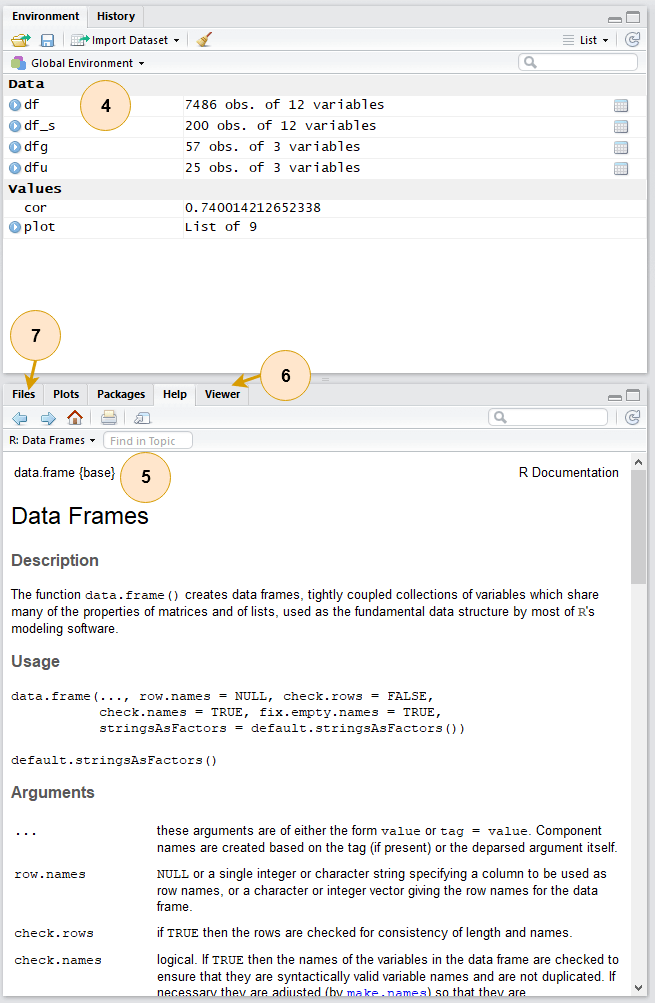
# To see a help page for a function (such as data.frame()) run either of:
help(data.frame)
?data.frame
# To see the arguments a function takes, run:
args(data.frame)
## function (..., row.names = NULL, check.rows = FALSE, check.names = TRUE, 
##     fix.empty.names = TRUE, stringsAsFactors = FALSE) 
## NULL

Making your own functions!

  • Use the function() function!
    • my_func <- function(agruments) {code}

Simple function: Add 2 to a number

add_two <- function(n) {
  n + 2
}

add_two(500)
## [1] 502

Slightly more complex function example

mult_together <- function(n1, n2=0, square=FALSE) {
  if (!square) {
    n1 * n2
  } else {
    n1 * n1
  }
}

mult_together(5,6)
## [1] 30
mult_together(5,6,square=TRUE)
## [1] 25
mult_together(5,square=TRUE)
## [1] 25

Example: Currency conversion function

FXRate <- function(from="USD", to="SGD", dt=Sys.Date()) {
  options("getSymbols.warning4.0"=FALSE)
  require(quantmod)
  data <- getSymbols(paste0(from, "/", to), from=dt-3, to=dt, src="oanda", auto.assign=F)
  return(data[[1]])
}
date()
## [1] "Sun Aug 15 23:41:31 2021"
FXRate(from="USD", to="SGD")  # Today's SGD to USD rate
## [1] 1.357472
FXRate(from="SGD", to="CNY")  # Today's SGD to CNY rate
## [1] 4.772041
FXRate(from="USD", to="SGD", dt=Sys.Date()-90)  # Last quarter's SGD to USD rate
## [1] 1.333589

Practice: Functions

  • This practice is to make sure you understand functions and their construction
  • Do exercises 4 and 5 on today’s R practice file:

End Matter

Wrap up

  • For next week:
    • Take a look at Datacamp!
      • Be sure to complete the assignment there
      • A complete list of assigned modules over the course is on eLearn
    • We’ll start in on some light analytics next week
  • Survey on the class session at rmc.link/420survey1

Packages used for these slides

Appendix: Getting data from WRDS

Data Sources

  • WRDS
    • WRDS is a provider of business data for academic purposes
    • Through your class account, you can access vast amounts of data
    • We will be particularly interested in:
      • Compustat (accounting statement data since 1950)
      • CRSP (stock price data, daily since 1926)
  • We will use other public data from time to time
    • Singapore’s big data repository
    • US Government data
    • Other public data collected by the Prof

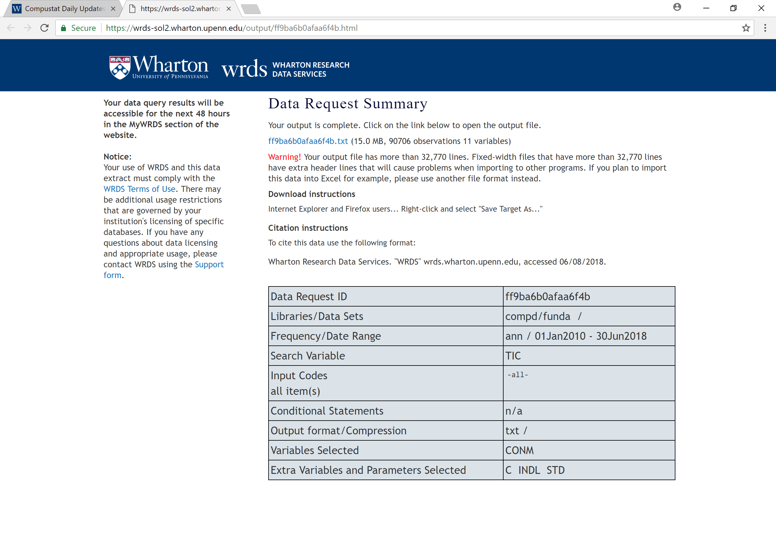
How to download from WRDS

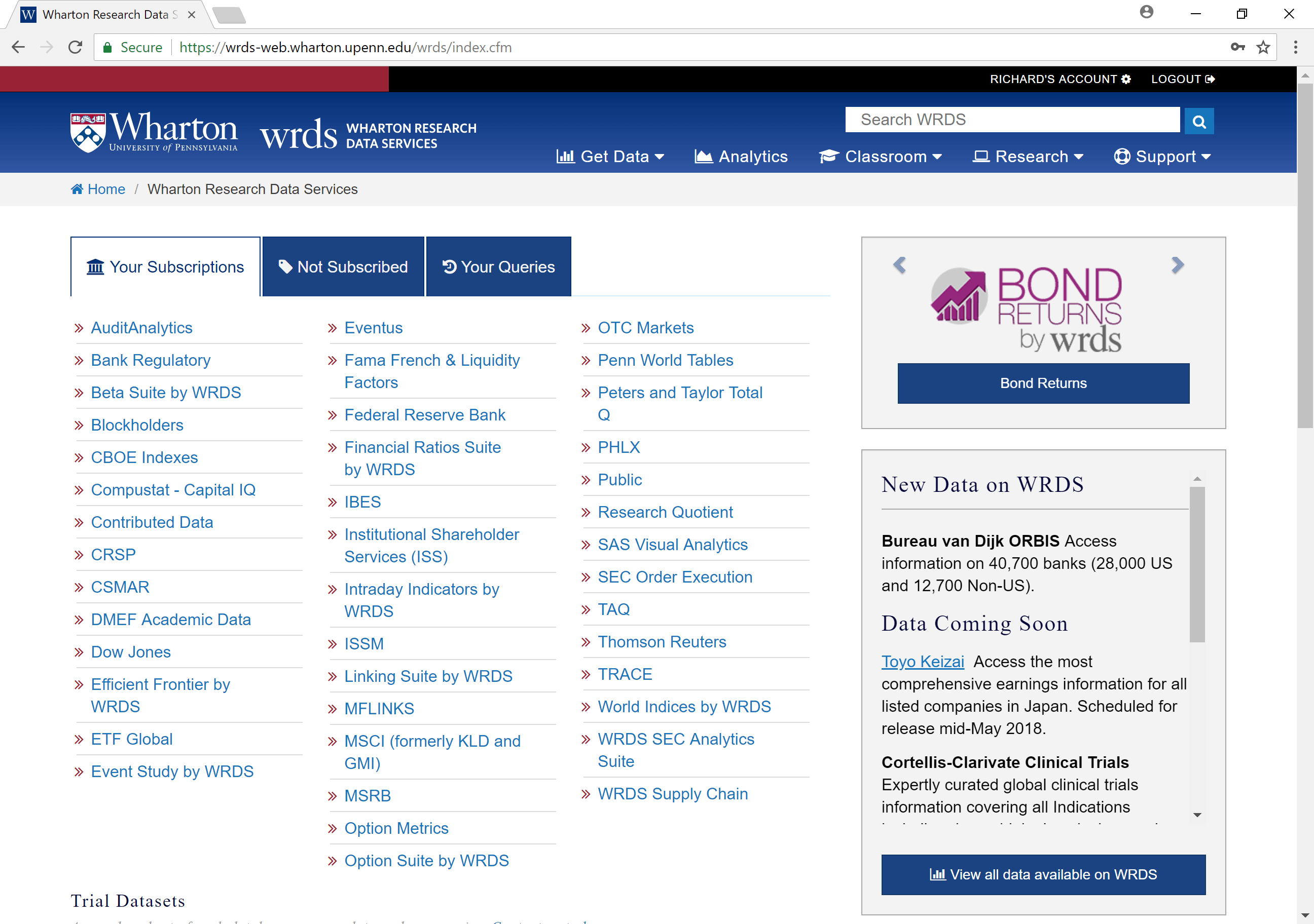
  1. Log in using a class account (posted on eLearn)
  2. Pick the data provider that has your needed data
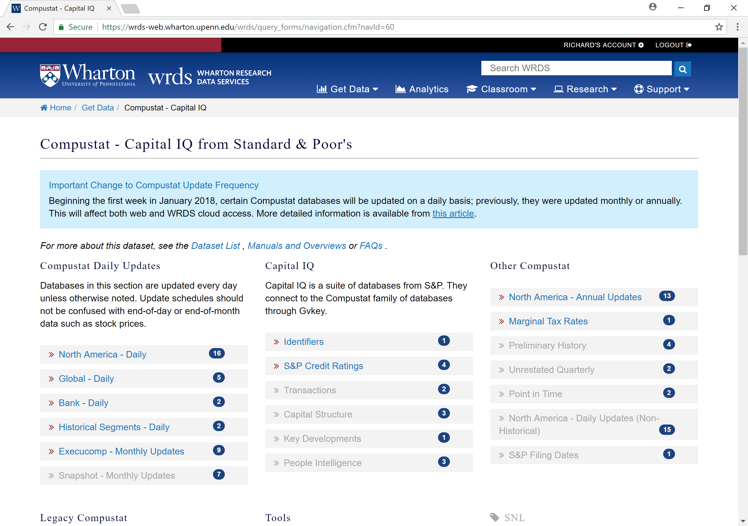
  3. Select the data set you would like (some data sets only)
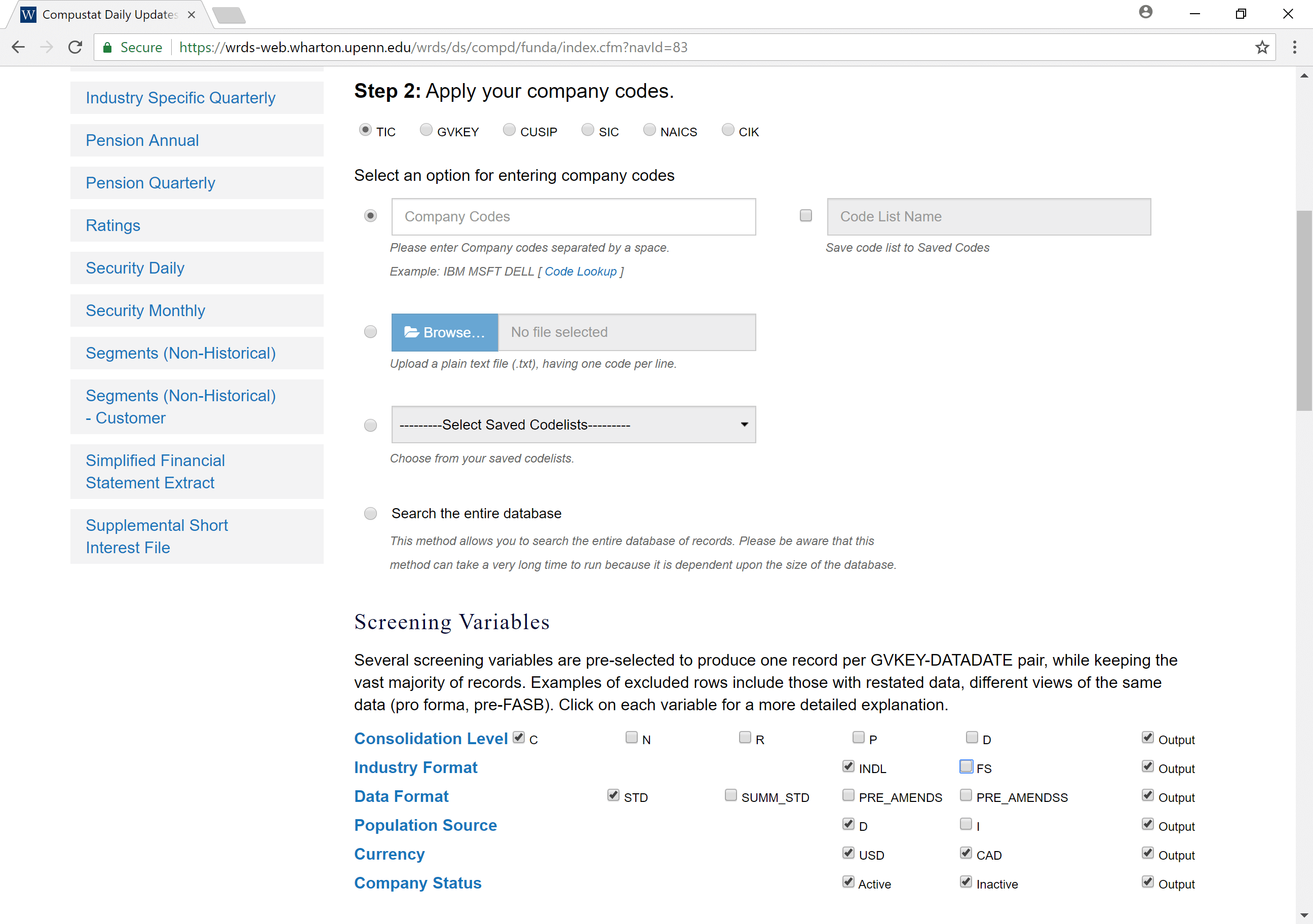
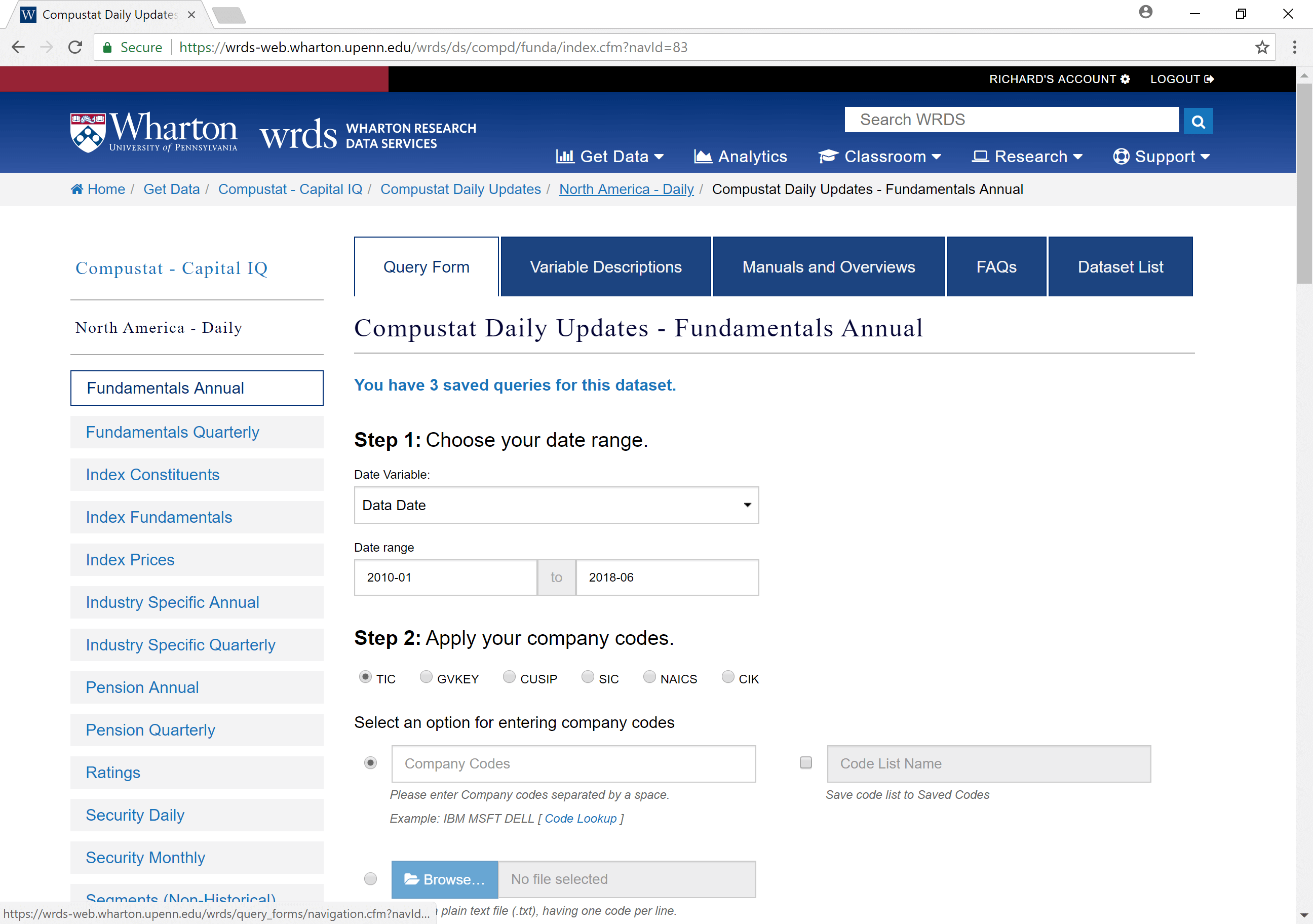
  4. Apply any needed conditional restrictions (years, etc.)
    • These can help keep data sizes manageable
      • CRSP without any restrictions is >10 GB
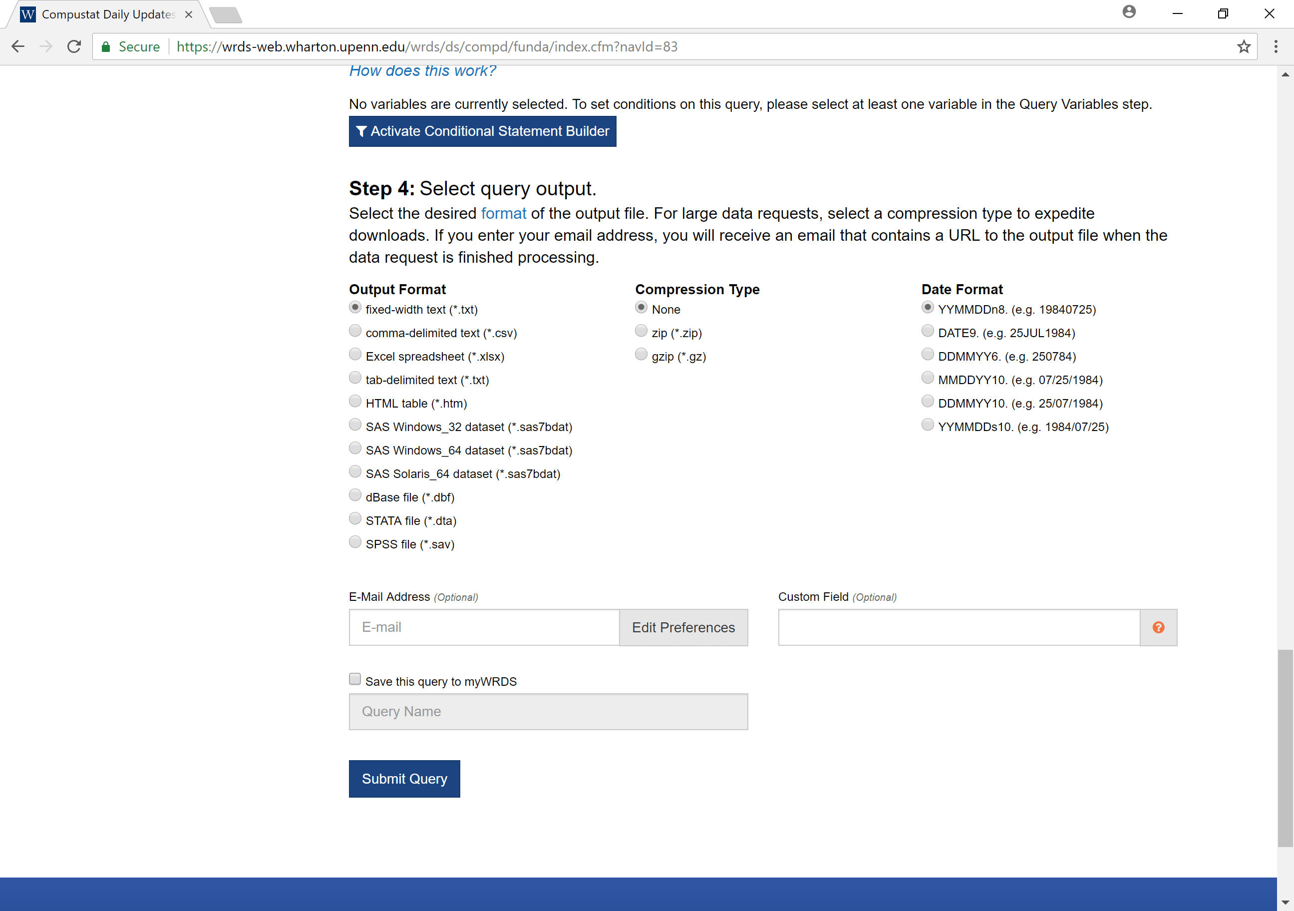
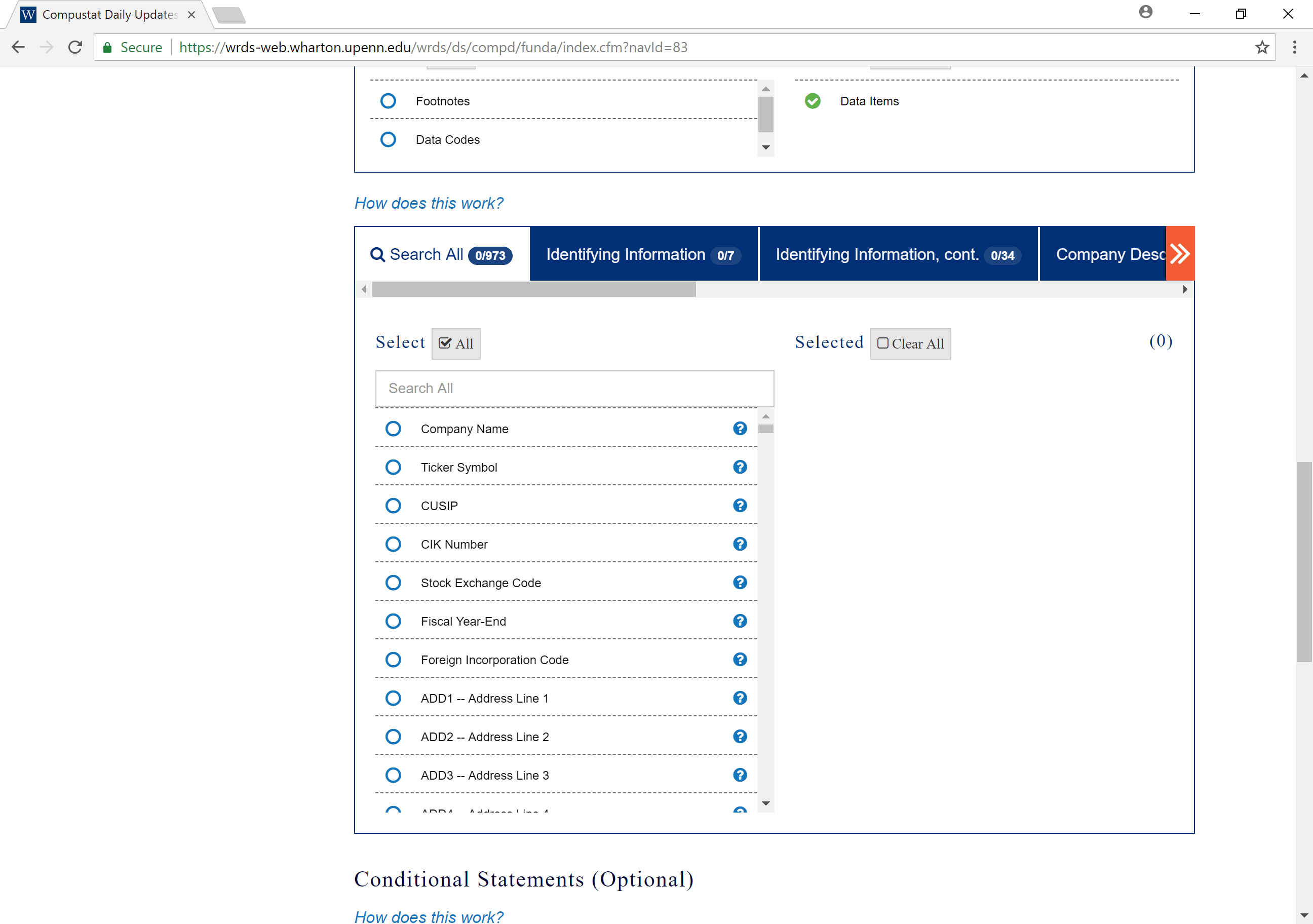
  5. Select the specific variables you would like export
  6. Export as a csv file, zipped csv file (or other format)

Picture walkthrough for WRDS

Go to WRDS and sign in

Pick a data provider, e.g. “Compustat - Capital IQ”

Pick a data set, e.g. “North America - Daily”

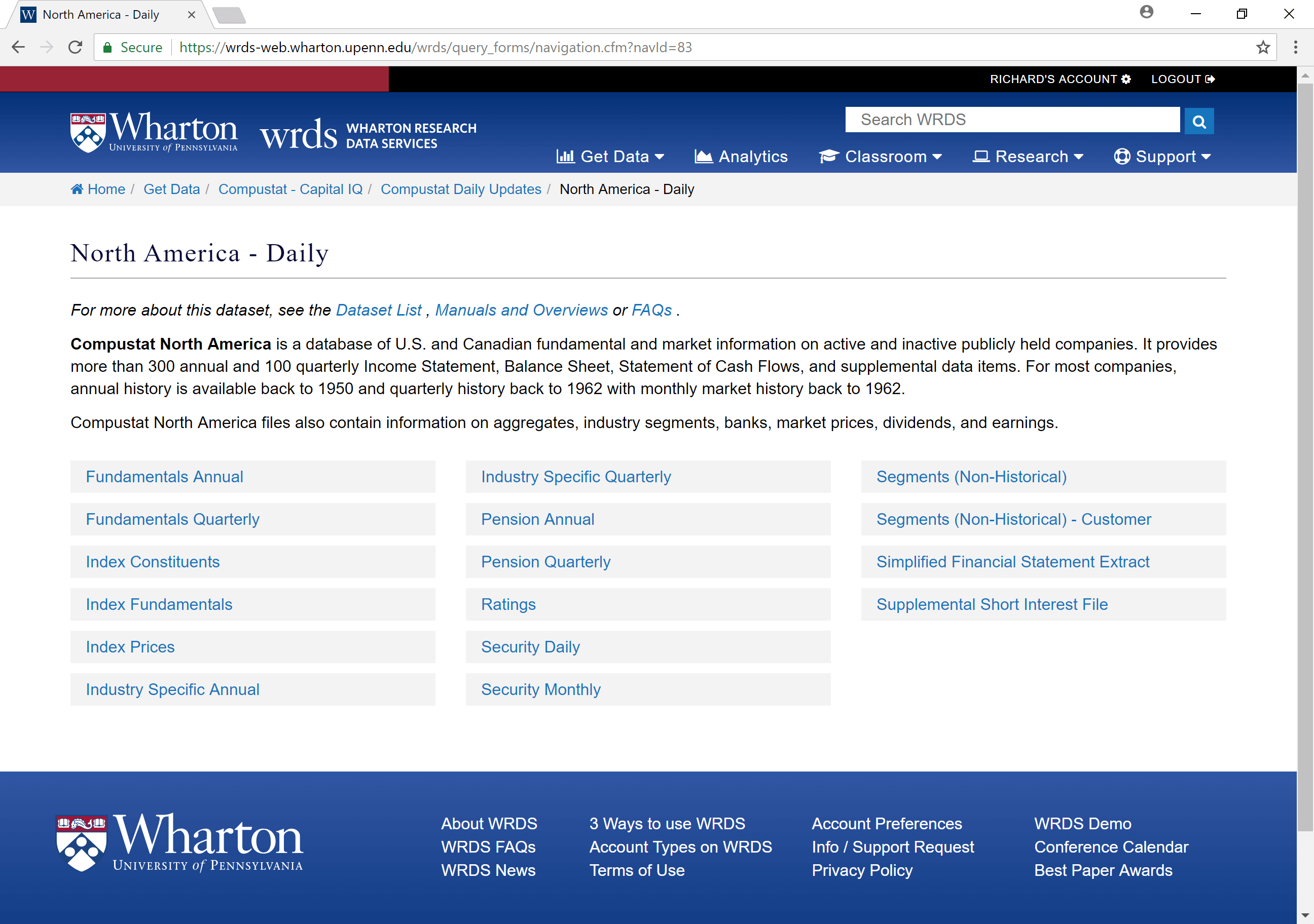
Pick a data set, e.g. “Fundamentals Annual”

Selecting data: Time range

Selecting data: Companies and data format

Selecting data fields

Select output formats

Wait for the data to be prepared
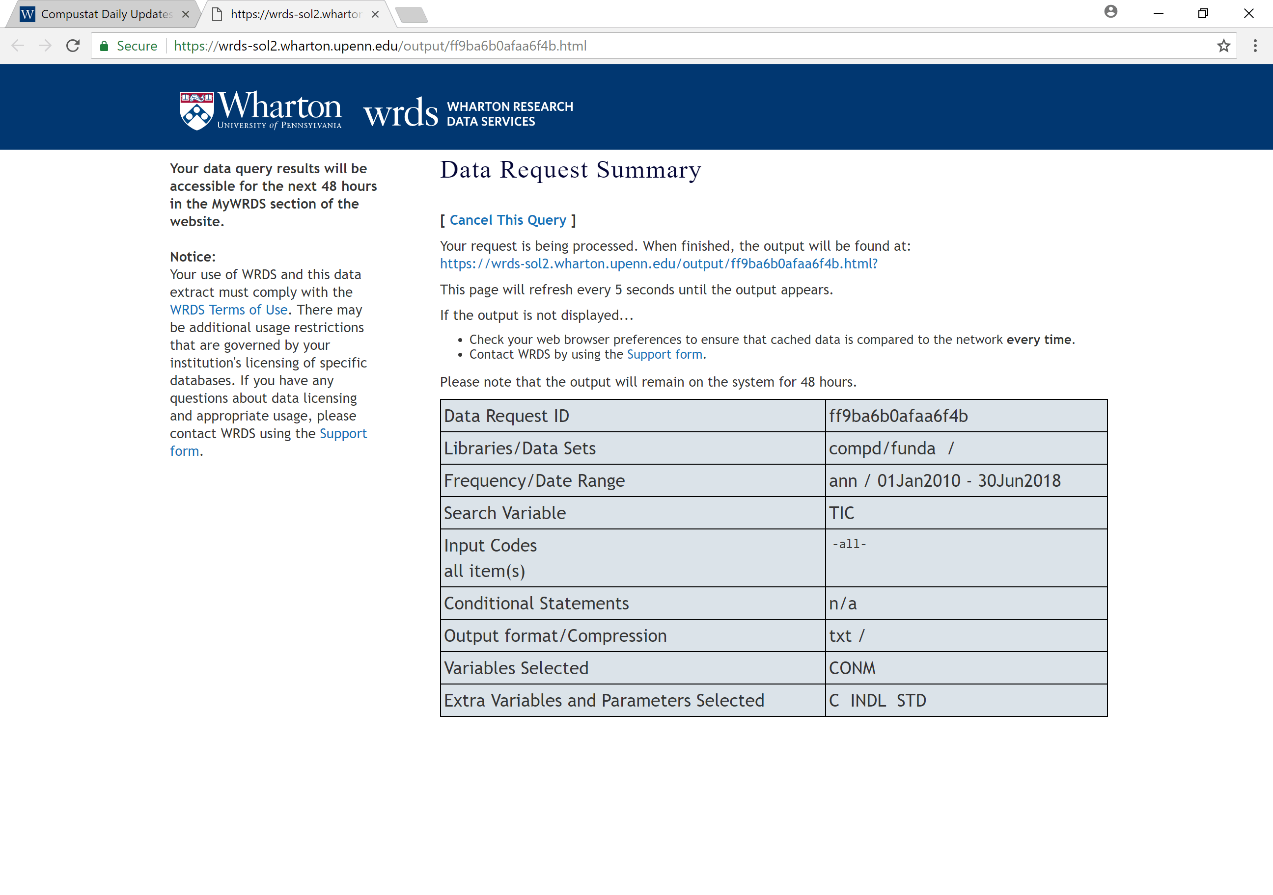
Download the data!